This section moves from discussing hypothetical risks to looking at what actually happens when remediation steps are tested in real-world settings.
Learning Objectives
By the end of this chapter, students will be able to:
-
1. Position digital twin simulation as simulation analytics within the SEAS-8414 taxonomy and explain how it transforms prescriptive recommendations into validated remediation plans.
-
2. Explain why remediation in OT/IoT environments requires simulation rather than direct deployment, and articulate the three failure modes that simulation prevents.
-
3. Describe the Docker-based architecture of the Breakwater digital twin system: how scan data is converted into Docker containers and bridge networks that replicate the production network.
-
4. Trace the construction and deployment of a digital twin from scan data through profile mapping, Docker bridge creation, container startup, and traffic injection to a running twin environment.
-
5. Design a scenario engine that replays attack paths and pentest campaigns against the twin, and explain how deterministic hashing enables reproducible simulation.
-
6. Implement a remediation simulation with checkpoint/rollback semantics and explain why immutable pre-remediation snapshots are indispensable for a safe comparison.
-
7. Calculate the breakwater risk score (BRS) delta for a remediation plan and explain the risk scoring components: port exposure, open firewall rules, default credentials, and vulnerability count.
-
8. Detect chain failures from remediation actions using dependency graph traversal and explain three dependency inference heuristics: firewall rules, MQTT broker patterns, and gateway dependencies.
-
9. Apply a Monte Carlo simulation to estimate the probability distribution of remediation outcomes under parameter uncertainty.
-
10. Design a patch-ordering algorithm that satisfies a maximum offline constraint while minimizing the total remediation time.
-
11. Replay captured network traffic against the twin Docker containers to validate that remediation does not break authorized communications, and explain the before/after fidelity comparison methodology.
-
12. Validate remediation plans against IEC 62443 and NIST SP 800-82 compliance controls, and explain which specific controls (SR-1.1, SR-2.1, SR-3.4, SR-5.1, AC-3, AC-4, IA-5, SI-2, AU-2) are checked and why each matters for industrial control system security.
-
13. Validate zero-disruption remediation using the four-check validation model: port reachability, orphaned firewall rules, bridge container counts, and critical infrastructure connectivity.
-
14. Explain behavioral drift detection using the KL-divergence and the Jensen-Shannon divergence, and describe how drift invalidates the twin assumptions.
-
15. Trace the water treatment plant scenario from vulnerability discovery through Docker twin construction, traffic replay validation, IEC 62443/NIST 800-82 compliance scoring, patch ordering optimization, remediation simulation, and validated deployment.
Agentic Lens
This chapter stresses the need to be careful before making remediation changes. Instead of using simple rules, every proposed fix should be backed up by simulation, policy checks, and careful analysis of dependencies before it is used in a real environment.
Implementation Note: Proposed remediation actions are evaluated through simulation before execution. The simulation is an approximation of the physical system. A proposed fix that works in simulation may still fail on the real device due to timing, state, or environmental differences.
-
Agent role: Turn a remediation idea into a validated execution plan.
-
Observations: Scan results, attack paths, traffic traces, device dependencies, compliance controls, and twin fidelity signals.
-
Tools: Digital twin builder, replay engine, checkpoint manager, compliance checker, Monte Carlo simulator, and patch scheduler.
-
State: Current twin version, drift score, open hypotheses, dependency graph, rollback points, and maximum offline budget.
-
Verifier: Replay success, health checks, compliance gates, cascading-failure analysis, and fidelity thresholds.
-
Guardrails: A digital twin exhibiting low fidelity should not be relied upon for final decision-making. Furthermore, a positive Breakwater Risk Score (BRS) delta alone is insufficient to inform remediation decisions.
-
It's important to remember that relying too much on the digital twin, without checking its assumptions, can give a false sense of security. Simulations that seem to work may not always lead to good results in real production environments.
Threat Model and Assumptions
This chapter models remediation risk as an approximation of production, not a perfect duplication.
-
Threat model: The defender aims to prevent self-inflicted outages while reducing the attacker's opportunities through patching, segmentation, credential rotation, or protocol changes.
-
Threat model: The attacker benefits whenever the defender is forced to choose between living with known exposure and applying a change that may destabilize operations.
-
Assumption: The twin inherits its structure from earlier discovery, enrichment, vulnerability, and attack-path outputs. If those inputs are wrong, the twin can be confidently wrong in the same direction.
-
Assumption: Dockerized or profile-based twins capture many important dependencies, but not every vendor quirk, timing edge case, physical process interaction, or undocumented control-plane dependency.
-
Assumption: Simulation results are decision support, not deployment guarantees. The chapter uses them to rank and screen candidate actions before live approval.
-
Scope boundary: This chapter does not assert that a digital twin can certify safety for high-consequence medical, industrial, or life-safety modifications without supplementary domain-specific review. In such cases, simulation results should always be escalated to domain experts for review before any remediation actions are implemented. Criteria for escalation include: when the remediation involves control systems that could directly impact human safety; when simulation indicates unexpected or high-severity cascading failures; when physical process behaviors fall outside modeled assumptions; or when planned changes could disrupt integrated industrial processes. Students should recognize these triggers and ensure direct coordination with process engineers, safety officers, or other relevant specialists, treating simulation analytics as a decision-support tool rather than a final authority in high-consequence environments.
-
It is essential to recognize that the simulation tools described do not provide formal safety guarantees. In contrast to formal verification, which mathematically verifies the safety of all system states, simulation analytics evaluate only modeled behaviors, dependencies, and interactions, potentially overlooking certain edge cases or unexpected behaviors. Achieving comprehensive formal verification for operational technology networks remains difficult due to device heterogeneity, proprietary protocols, and incomplete specifications. The current best practice is to employ simulation to identify probable hazards, while acknowledging that full safety certification necessitates additional domain-specific modeling and exhaustive state checking tools. For further information on integrating simulation with formal methods, consult research on co-simulation frameworks and runtime verification for cyber-physical systems. To promote operational transparency and regulatory compliance, organizations should implement a formal escalation process. Teams are advised to document all escalation triggers identified during planning or simulation, including proposed remediation actions, simulation outcomes, and supporting rationale. This documentation should be promptly communicated to relevant experts or authorities using checklists, incident management systems, or standardized protocols. Maintaining comprehensive records supports compliance demonstration, informed decision-making, and efficient reviews and audits.
6.1 Analytics Context: Simulation Analytics
Chapters 1 through 5 established an analytical process that addressed progressively complex questions. Discovery identified the devices present in the network. Enrichment determined the characteristics of those devices. Vulnerability assessment evaluated their security weaknesses. Attack graphs mapped potential attacker pathways, and autonomous penetration testing assessed which attacks are feasible. While each chapter provided valuable insights, none addressed the central operational question: what are the consequences when remediation is implemented? Addressing this simulation question requires a distinct analytical approach compared to previous chapters.
| Descriptive | What devices exist on the network? | Ch 1: Discovery |
|---|---|---|
| Diagnostic | What are these devices doing? | Ch 2: Enrichment, fingerprinting |
| Detective | What vulnerabilities do they have? | Ch 3: CVE, OpenVAS, Nuclei |
| Predictive | What attack paths are likely? | Ch 4: Attack graphs, BRS scoring |
| Prescriptive | What offensive tests should we run? | Ch 5: Autonomous pentest |
| Simulation | What happens if we apply this fix? | Ch 6: Digital twin |
| Autonomous | Act on it | Ch 7-12: Quantum to remediation |
Table 6.1. Analytics taxonomy mapped to the 12-chapter course structure.
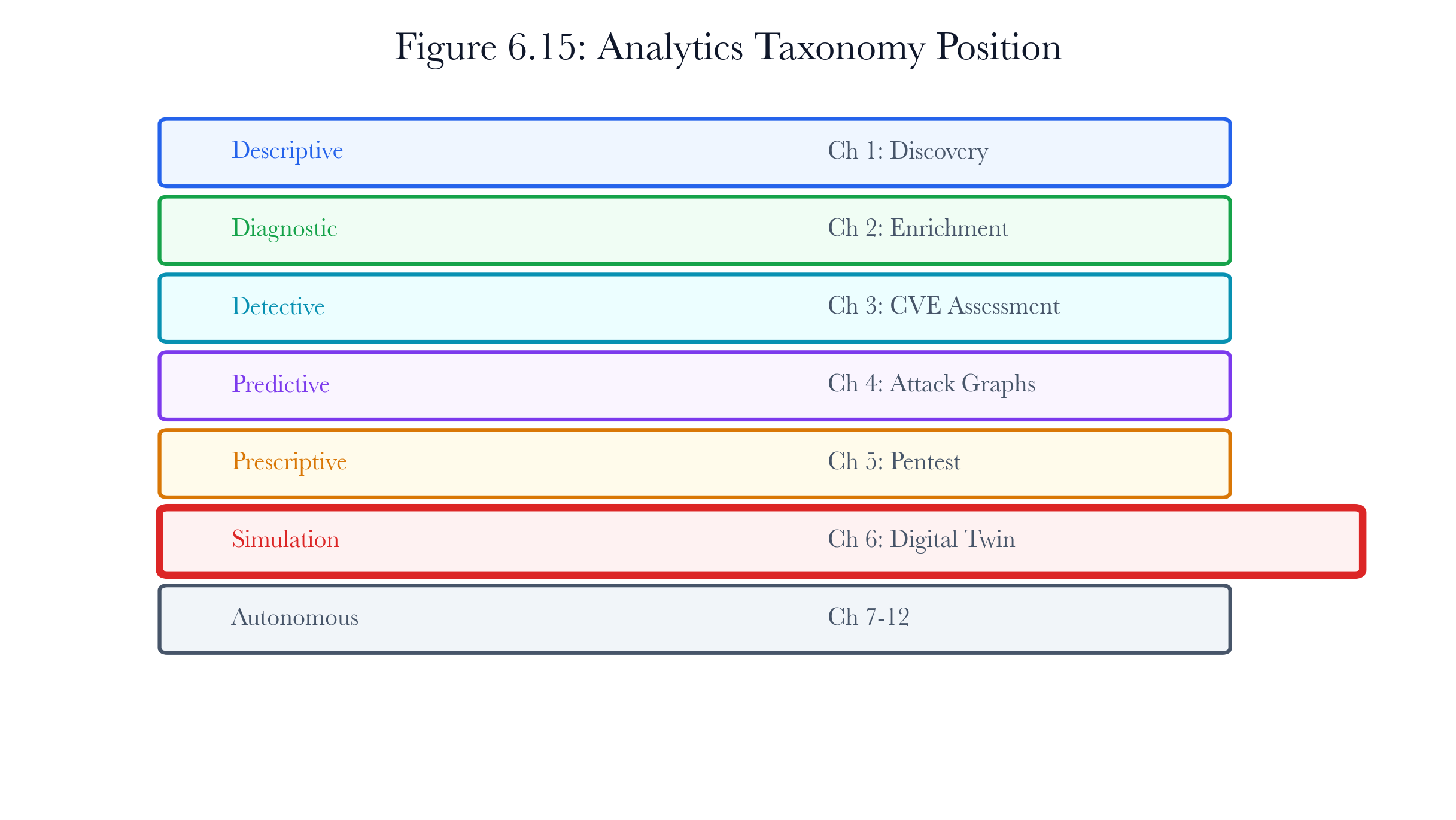
Figure 6.1: Analytics taxonomy for simulation. Digital twin analytics tests the consequences of remediation after prescriptive pentest evidence identifies what should be fixed.
Simulation analytics is fundamentally distinct from prescriptive analytics. While prescriptive analytics recommends specific actions, simulation analytics evaluates the outcomes of those actions. For example, a prescriptive system may recommend patching 40 programmable logic controllers (PLCs), whereas a simulation system examines the optimal patching order, concurrency constraints, and potential failures, such as the impact if PLC-17 requires twice the expected reboot time.
The outcome of this chapter is a validated remediation plan that includes quantified risk reduction, identification of cascading failures, and a rollback checkpoint for potential production failures. This plan is tested in an environment that replicates the production network’s topology, device profiles, firewall rules, and service dependencies. Such comprehensive testing distinguishes simulation analytics from prescriptive approaches.
6.1.1 The Remediation Gap
Security teams are good at finding vulnerabilities, but the main challenge is fixing them without causing new problems for operations.
The problem isn't a lack of skill—it's a structural challenge. Tools like vulnerability scanners and penetration testers can tell you that “CVE-2023-3595 affects PLC-17,” but they don't show what happens to the chemical dosing loop if PLC-17 reboots. They also don't reveal if PLC-23, which depends on PLC-17, will have issues, or if changing the SCADA VLAN's segmentation will disrupt the historian's data collection.
The remediation gap is the difference between knowing what needs to be fixed and figuring out how to fix it safely. In IT, this gap is usually small—patching a web server and rolling back if needed is simple. But in OT and IoT, the gap is much bigger. One mistake can cause chemical spills, equipment overheating, or safety incidents that can't be undone.
-
In OT networks, dependencies are often hidden and hard to see. Unlike IT environments, where connections are usually well-documented, OT devices are linked by physical processes, shared wiring, and timing details that don't show up in network diagrams.
-
In OT environments, there are rarely chances to take systems offline for maintenance. Unlike IT, where you can take a web app down during off-hours, critical systems like water treatment plants have to run all the time. Simulation helps by letting teams safely test fixes, find hidden dependencies, and spot possible failures before they affect real systems. For example, simulation might show that rebooting two PLCs at once could disrupt chemical dosing accuracy—a risk you might not notice just by planning.
6.1.2 Why Not Just Use a Staging Environment?
IT organizations routinely deploy staging environments for pre-production testing. Why not apply the same approach to OT networks?
Three reasons make staging impractical for the environments addressed in this chapter.
First, OT devices are expensive and specialized. A staging environment for 40 PLCs controlling chemical dosing would require 40 additional PLCs, 40 I/O modules, and process simulation hardware. The capital cost alone would exceed the security budget.
Second, physical process coupling cannot be staged. The PLCs do not just run firmware; they control valves, pumps, and sensors through analog and digital I/O. Staging firmware without the physical process tests only half the system.
Third, staging environments often become outdated over time. They aren't maintained as closely as production, so differences build up and the test system no longer matches the real one. A digital twin built from actual production scan data avoids this problem. Still, it's not always a replacement for staging. For enterprise web apps with clear deployment processes, staging is still best. But for complex OT networks with many devices and hidden dependencies, the digital twin lets you test changes when staging isn't practical.
6.2 Digital Twin Concepts for Network Security
6.2.1 What Is a Network Digital Twin?
A digital twin, in the broadest sense, is a software model that mirrors a physical system closely enough to predict the system’s behavior under changed conditions. The concept originated in manufacturing, where digital twins of turbines, aircraft engines, and production lines enable engineers to simulate maintenance procedures, test design changes, and predict remaining useful life without stopping the physical equipment.
A digital twin for a network applies the same principle to its infrastructure. It models devices, connections, firewall rules, and service dependencies of a production network in a virtual environment where changes can be tested safely.
The Breakwater digital twin is not a full-fidelity network emulator. It does not replicate packet-level timing, protocol state machines, or physical I/O behavior. What it does replicate is the topology, device profiles, firewall rule set, and service dependency structure. That level of fidelity is sufficient for the simulation questions this chapter addresses: patch ordering, firewall rule changes, network segmentation, credential rotation, and service disablement.
6.2.2 Twin Fidelity Spectrum
Digital twins exist on a spectrum of fidelity. At the low end, a twin might be nothing more than a topology graph with device labels. At the high end, it might be a cycle-accurate hardware emulator running actual PLC firmware. The Breakwater twin sits in the middle of this spectrum, at what we call “structural fidelity.”
| Topological | Nodes and edges only | Connectivity analysis | Partial |
|---|---|---|---|
| Structural | Topology + services + firewall rules + dependencies | Remediation simulation | Yes |
| Behavioral | Structural + protocol state machines + traffic patterns | Anomaly detection | Partial (drift detection) |
| Physical | Behavioral + I/O simulation + process coupling | Safety verification | No |
Table 6.2. Digital twin fidelity spectrum. Breakwater operates at the structural level with partial behavioral capability through drift detection.
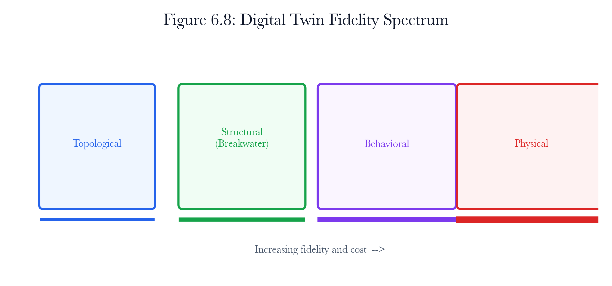
Figure 6.2: Digital twin fidelity spectrum. The Breakwater twin sits at structural fidelity, which is sufficient for remediation and dependency analysis but falls short of full physical-process emulation.
Structural fidelity is the right level for remediation simulation because most questions are about structure. For example, if you want to know whether turning off Telnet on PLC-17 will break its connection to PLC-23, you need to look at firewall rules and service dependencies, not packet timing. In the same way, checking if patching three PLCs at once will go over safety limits is about task order, not protocol timing details.
Higher fidelity would help with safety-critical checks, but it would also need PLC firmware images, I/O setup data, and process models that most security teams don't have. The structural twin, on the other hand, can be built just from scan data the security team already has.
6.2.3 The Twin Is a Running Docker Environment
This point deserves emphasis because it separates the Breakwater twin from purely abstract graph models. The digital twin is not a diagram or data structure on a dashboard. When deployed, it runs a Docker environment with real bridge networks, containers, and IP addresses. Each discovered device becomes a Docker container running an IoT simulation image exposing the same ports as the production device. Each production subnet becomes a Docker bridge network with the same isolation boundaries. The twin topology is literally a Docker Compose deployment you can see with docker ps.
The TwinDockerManager class handles this translation. It uses the Docker SDK for Python (docker.from_env()) with all Docker API calls wrapped in asyncio.to_thread() so the scan pipeline is never blocked by container operations:
# From apps/api/app/scanning/digital_twin/docker_manager.py
class TwinDockerManager:
async def create_network(self, name: str, subnet: str) ->str:
"Create a Docker bridge network with IPAM configuration."""
def _create():
- ipam_pool = docker.types.IPAMPool(subnet=subnet)
ipam_config = docker.types.IPAMConfig(pool_configs=[ipam_pool])
network = client.networks.create(
name, driver="bridge", ipam=ipam_config,
)
return network.I'd
return await asyncio.to_thread(_create)
async def create_container(self, image, name, network, ip, ports, environment):
"Create and start a container on the specified bridge network."""
def _create():
networking_config = client.api.create_networking_config(
{network: client.api.create_endpoint_config(ipv4_address=ip)}
)
container = client.containers.create(
image, name=name, detach=True,
ports=ports, environment=environment,
networking_config=networking_config,
)
container.start()
return container.I'd
return await asyncio.to_thread(_create)
The deployment sequence is: (1) create Docker bridge networks for each subnet, (2) start a container per device with the correct image, IP, port bindings, and environment variables, (3) inject traffic between containers to verify connectivity. Containers receive environment variables identifying their twin context (TWIN_ID, ORIGINAL_IP, DEVICE_TYPE), so simulation images can adapt behavior based on the production device they represent. Why not GNS3 or EVE-NG? Three reasons. First, Docker containers start in under a second, making twin deployment fast enough to integrate into the scan pipeline without a separate provisioning step. Second, Docker bridge networks enforce real L2/L3 isolation, so firewall rules and segmentation tested on the twin behave the same way in production Docker deployments. Third, the same IoT simulation images used in the IoT-sim lab environment (the 22-device simulation network from make IoT-sim-up) serve double duty as twin device proxies, meaning the simulation images are already tested and maintained.
The twin also supports a pure simulation mode for environments without Docker (CI pipelines, restricted workstations). In this mode, topology analysis, scenario execution, remediation simulation, and cascade detection work identically, but no containers start. Pure simulation mode lacks live network stack emulation or protocol-level validation; responses are generated synthetically rather than through container-based services. As a result, traffic replay fidelity, behavioral testing, and service interaction checks are limited. Results should be interpreted as analytical guidance rather than verified operational predictions. Docker deployment enhances active testing but is not required for analytical queries.
6.2.4 The Twin Lifecycle
The digital twin follows a five-stage lifecycle:
-
Build. Scan data is transformed into a twin topology: devices mapped to simulation profiles, subnets modeled as Docker bridge networks, and firewall rules inferred from open ports and traffic patterns.
-
Deploy. The twin topology is instantiated as live Docker containers for active testing. Each device becomes a running container; each subnet becomes a Docker bridge. Alternatively, the twin operates in pure simulation mode for analytical queries.
-
Scenario. Attack paths and pentest campaigns from Chapters 4 and 5 are replayed against the twin to establish a baseline threat model. Traffic from production can be replayed against the containers to verify fidelity.
-
Remediate. Remediation actions are applied to the twin: patches, credential rotations, firewall changes, and network segmentation. Each action is previewed with risk scoring, cascading failure detection, and compliance validation with IEC 62443 / NIST 800-82.
-
Validate. The remediated twin is checked against zero-disruption criteria and compliance frameworks. If validation passes, the remediation plan is promoted to production. If it fails, the twin is rolled back to the pre-remediation checkpoint.
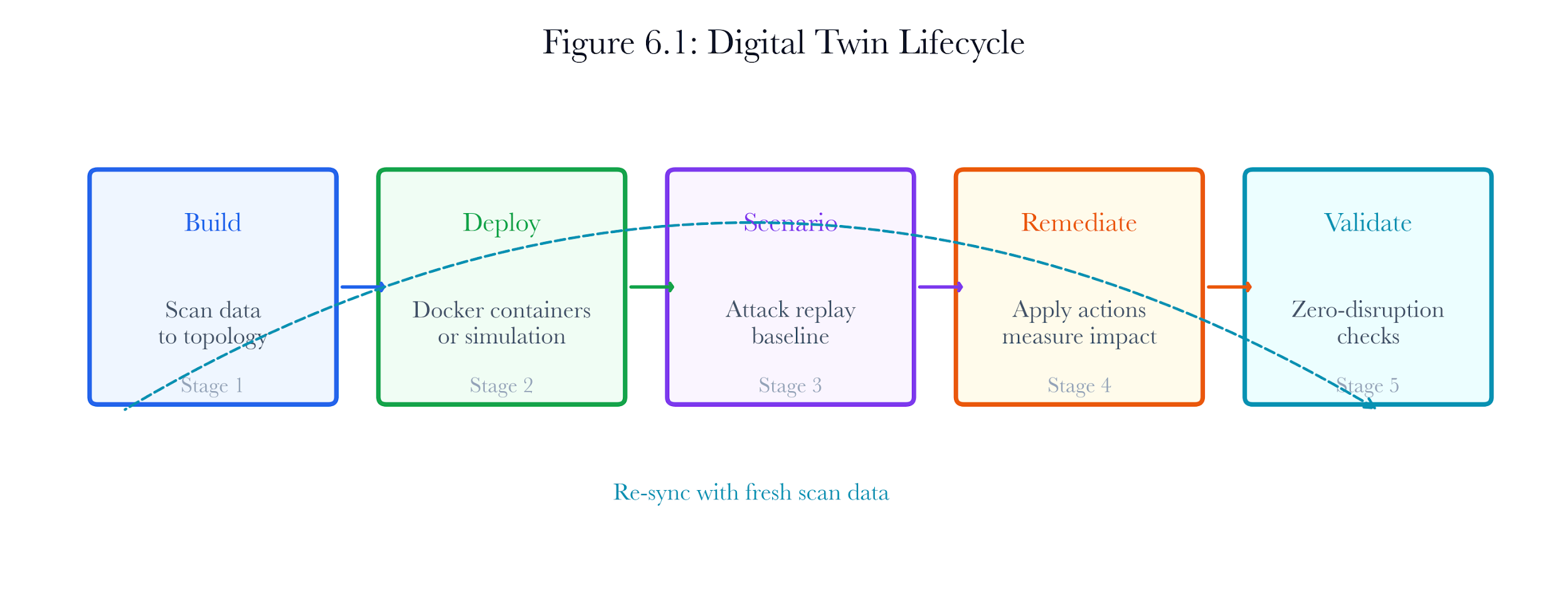
Figure 6.3: Digital twin lifecycle. Five stages from scan data ingestion through a validated remediation plan.
This lifecycle keeps going as the production network changes. The twin should be updated with new scan data, tested with new scenarios, and used to try out new remediation plans. It's a living model that grows with the real network. In practice, update the twin regularly: after each vulnerability scan, after big network changes, or before planned fixes. Also update it if you get drift alerts, during incident response, or after compliance checks. Keeping the twin up to date makes it a reliable tool for making decisions.
To help teams operationalize lifecycle management, the following checklist summarizes the recommended process for updating the twin:
1. Collect up-to-date scan data from the production network.
2. Validate the scan results for completeness and accuracy.
3. Synchronize the digital twin with the current scan data, applying incremental changes when possible.
4. Test the twins' fidelity (e.g., replay recent production traffic and check for behavioral match).
5. Run new scenarios or remediation simulations as required.
6. Review drift detection metrics to confirm the model remains aligned with production.
7. Document any updates, issues, or validation results for audit and compliance purposes.
By following these steps, you keep the digital twin accurate and make sure it keeps giving useful, risk-based advice for protecting the network.
6.3.1 The Build-and-Deploy Pipeline
The twin construction pipeline transforms raw scan results into a structured topology and, when Docker is available, deploys it as a running container environment. The entry point is the NetworkDigitalTwin class:
# From apps/api/app/scanning/digital_twin/twin_builder.py
twin = NetworkDigitalTwin()
topology = twin.build_from_scan(scan_id, hosts)# Step 1-4: build topology
topology = await twin.deploy(topology.twin_id)# Step 5: start containers
The build proceeds in five steps:
-
Profile mapping: Each host is mapped to an IoT simulation profile using the DeviceProfileMapper. The mapper uses a three-tier resolution strategy: direct device-type lookup, port-based inference, and service-name hinting.
-
Subnet grouping: Hosts are grouped by /24 subnet prefix. Each group becomes a SubnetBridge – a Docker bridge network with IPAM configuration that mirrors the production broadcast domain.
-
Firewall rule inference: Open ports on each host generate inbound allow rules. Inter-host dependencies (such as IoT sensors communicating with MQTT brokers) generate cross-host rules.
-
Topology assembly: Devices, bridges, and firewall rules are composed into a TwinTopology object that serves as the simulation substrate for all subsequent operations.
-
Docker deployment: The deploy() method creates Docker bridge networks for each subnet, then starts a container per device. Each container runs an IoT simulation image (breakwater-iot-sim-{profile}: latest) configured with the device’s original IP, type, and port bindings. Container IPs are assigned sequentially within each bridge subnet, starting at .2 (the .1 address is reserved for the bridge gateway).
# From twin_builder.py — deploy()
async def deploy(self, twin_id: str) -> TwinTopology:
# 1. Create Docker bridge networks
for bridge in topology.bridges:
nid = await self._docker.create_network(
bridge.network_name, bridge.subnet_cidr
)
# 2. Start a container per device
for the device in the topology. devices:
image =f"breakwater-iot-sim-{device.profile_name}:latest"
env = {"TWIN_ID": twin_id, "ORIGINAL_IP": device.device_ip,
"DEVICE_TYPE": device.device_type}
cid = await self._docker.create_container(
image=image, name=container_name,
network=bridge_name, ip=container_ip,
ports=port_bindings, environment=env,
)
device.container_id = cid
device.container_status ="running" if cid else" failed."
topology.status = TwinStatus.deployed
After deployment, the twin is a set of running Docker containers that can receive real network traffic. The inject_traffic() method on TwinDockerManager executes docker exec commands inside containers to send HTTP requests (via curl) or raw TCP payloads (via nc) to other containers in the twin, verifying that connectivity and service behavior match production expectations.
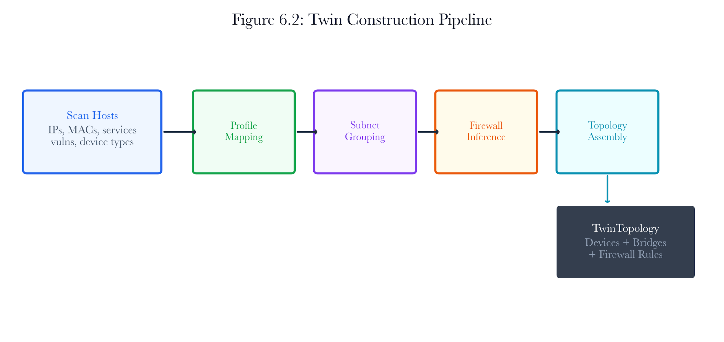
Figure 6.4: Twin construction pipeline. Five stages from raw scan hosts to running Docker containers.
6.3.2 Device Profile Mapping
The profile mapper translates real-world device diversity into a manageable set of simulation profiles. The Breakwater twin uses five profiles:
| camera-variant | 80, 554, 8080 | IP cameras, NVRs | Security cameras are monitoring the chemical storage area |
|---|---|---|---|
| rtsp-vuln | 554, 8554, 80 | NVRs, DVRs with RTSP | Video feeds from the treatment floor |
| http-debug | 80, 443, 8080 | Routers, switches, printers, NAS | SCADA HMI web interfaces, historian web dashboard |
| mqtt-device | 1883, 8883, 80 | Sensors, thermostats, IoT hubs | Chemical concentration sensors publishing to MQTT |
| telnet-vuln | 23, 80, 502 | PLCs, SCADA, HMIs, industrial | The 40 ControlLogix PLCs running Modbus on port 502 |
Table 6.3. IoT simulation profiles and their production mappings.
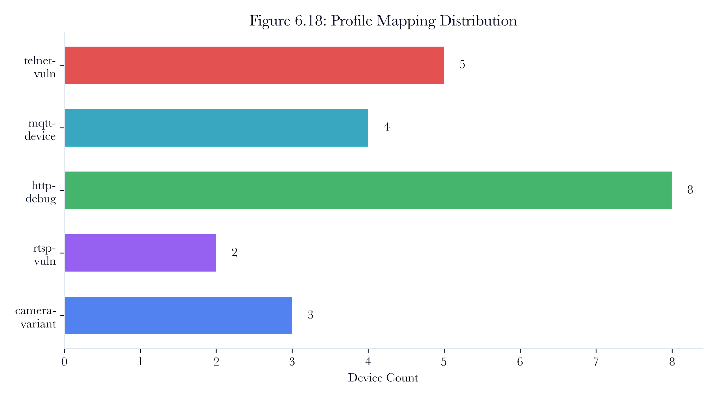
Figure 6.5: Device profile mapping. Device type, port evidence, and service-name hints map production assets to simulation profiles with explicit confidence.
The mapping uses three tiers of evidence, applied in priority order:
Tier 1: Device type: If Phase 3 fingerprinting identified the device type (e.g., “plc”), the mapper uses the DEVICE_TYPE_MAP dictionary for a direct lookup. This is the highest-confidence path because the device type was already inferred from multiple evidence sources in Chapter 2.
Tier 2: Port inference: If the device type is unknown, the mapper examines open ports. Ports 554 and 8554 strongly indicate RTSP (camera or NVR). Ports 1883 and 8883 indicate MQTT. Ports 23, 502, 102, and 47808 are used for industrial protocols. The priority order is RTSP > MQTT > industrial > HTTP, which reflects the specificity of each port as an identity signal.
Tier 3: Service name hinting: If port inference is inconclusive, the mapper checks service names from nmap enrichment data. A service named “modbus” maps to the industrial profile even if it runs on a non-standard port.
The confidence score for each mapping is calculated as:
confidence = 0.5 * (device_type_match) + 0.3 * (port_overlap) + 0.2 * (service_hint_match)
For the water treatment plant, this means the 40 PLCs get mapped with high confidence (0.7 to 1.0) because they have both a known device type (“plc”) and the expected port signature (23 + 502). The MQTT sensors get medium confidence (0.4 to 0.6) because they lack explicit device typing but expose the correct ports.
6.3.3 Subnet Bridge Construction
The twin models broadcast domain boundaries using Docker bridge networks. Each /24 subnet in the production network becomes a SubnetBridge:
# From twin_builder.py
subnet_groups =self._group_by_subnet(hosts)
bridges: list[SubnetBridge] = []
for idx, (subnet_key, group_hosts) in enumerate(subnet_groups.items()):
bridges. append(
SubnetBridge(
network_name=f"twin-{twin_id}-net{idx}",
subnet_cidr=f"{self._network_prefix}.{idx *16}/28",
gateway=f"{self._network_prefix}.{idx *16+1}",
container_count=len(group_hosts),
)
)
When only one subnet is present, the bridge uses a full /24 CIDR. When multiple subnets exist, each bridge gets a /28 slice, which provides 14 usable addresses per segment. This mapping preserves the subnet isolation boundaries from production while fitting within the twins’ address space.
For the water treatment plant, the network has three subnets: the SCADA control network (10.1.1.0/24) with the 40 PLCs and HMIs, the corporate IT network (10.2.0.0/24) with workstations and the historian, and the DMZ (10.3.0.0/24) with the perimeter firewall and remote access gateway. The twin creates three bridge networks to mirror this topology.
6.3.4 Firewall Rule Inference
The twin infers firewall rules from scan data rather than requiring manual configuration. Two categories of rules are generated:
Per-port inbound rules: For each open port on each host, the twin creates an allow rule from any source (0.0.0.0) to that host and port. These rules model the current exposure: if port 502 is open on PLC-17 in production, the twin reflects that exposure.
Inter-host dependency rules: The twin detects communication patterns that imply dependencies. Currently, the primary pattern is MQTT: if a host exposes port 1883 (MQTT broker) and another host has a device type of “sensor” or “thermostat,” the twin infers that the sensor depends on the broker and creates a directed allow rule between them.
# From twin_builder.py
# Inter-host: IoT devices -> MQTT brokers
for iot_ip in iot_devices:
for broker_ip in mqtt_brokers:
if iot_ip == broker_ip:
continue
for mport in (1883, 8883):
rules. append(
FirewallRule(
source_ip=iot_ip,
dest_ip=broker_ip,
dest_port=mport,
protocol="tcp",
action="allow",
inferred_from="mqtt_dependency",
)
)
For the water treatment plant, this inference creates rules from each chemical concentration sensor to the MQTT broker that aggregates dosing readings. Those dependency rules become critical during remediation simulation. If the broker is taken offline for patching, the sensors lose their data path, and the control system loses visibility into chemical concentrations.
The inference is deliberately conservative. It captures explicitly observable dependencies (open ports, MQTT patterns) rather than attempting to infer all possible communication. Undiscovered dependencies are a known limitation. Section 6.11 discusses how to address this gap with traffic replay and drift detection.
6.4 Network Topology Modeling
6.4.1 The TwinTopology Data Model
The complete twin topology is represented as a Pydantic model with four components:
# From apps/api/app/scanning/digital_twin/twin_schemas.py
class TwinTopology(BaseModel):
twin_id: str
scan_id: str
devices: list[TwinDevice]
bridges: list[SubnetBridge]
firewall_rules: list[FirewallRule]
created_at: str=""
status: TwinStatus = TwinStatus.building
Each TwinDevice carries the original scan evidence alongside its simulation profile:
class TwinDevice(BaseModel):
device_ip: str
profile_name: str
container_id: str|None=None
container_status: str="pending."
mapped_ports: dict[int, int]
original_services: list[dict[str, Any]]
device_type: str="unknown."
hostname: str="”
The original_services field preserves the full enrichment data from Phase 2: service names, versions, banners, vulnerability lists, and credential status. The remediation simulator consumes this data to calculate risk scores and detect cascading failures.
6.4.2 Topology as a Graph
Although the data model stores the topology as flat lists, the logical structure is a directed graph. Devices are nodes. Firewall rules are edges. The direction of each edge encodes the allowed traffic flow: a rule from sensor A to broker B means A can initiate connections to B, not the reverse.
This graph-architecture supports three key analytical operations:
-
Blast radius calculation: Given a set of compromised nodes, how many additional nodes are reachable through the allowed firewall rules? This is a breadth-first traversal from the compromised set, following edges in the allowed direction.
-
Dependency analysis: Given a node being taken offline for remediation, which other nodes lose a service they depend on? This is a reverse traversal: find all nodes with edges pointing to the offline node.
-
Segmentation analysis: Given a proposed firewall rule change, which existing traffic flows would be blocked? This requires comparing the pre-change and post-change edge sets.
Implementation Note: Firewall rule changes are proposed by the simulation engine. Before applying any rule to production infrastructure, validate it against the live traffic capture and confirm it does not block legitimate control-plane communication.
For the water treatment plant, the topology graph makes the PLC dependencies explicit. PLC-17 has inbound Modbus (port 502) connections from the HMI, outbound MQTT connections to the data broker, and a setpoint coordination link to PLC-23. Taking PLC-17 offline for patching breaks all three connections. The graph makes that visible before the patch is applied.
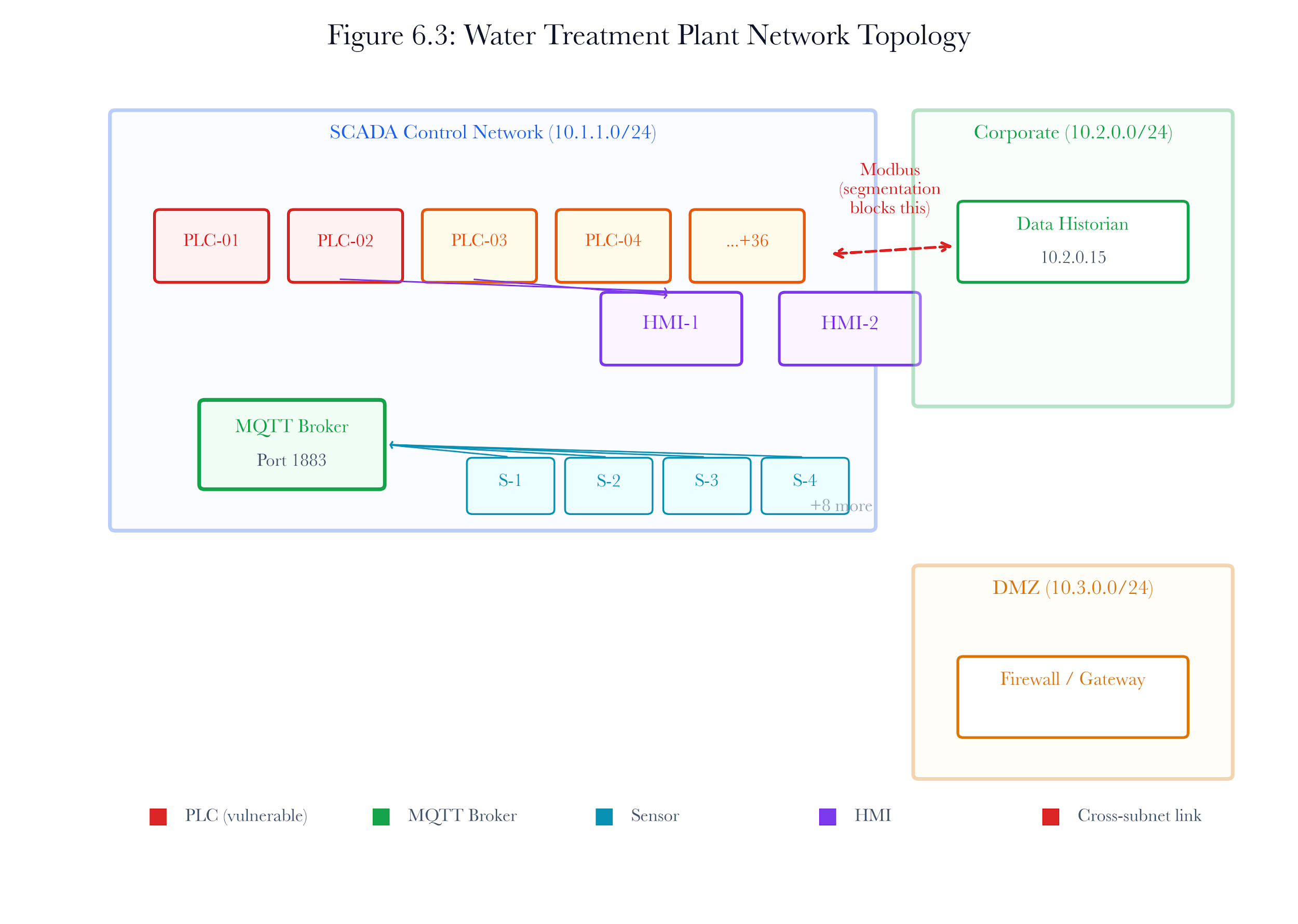
Figure 6.6: Water treatment plant topology as a directed graph. PLCs, sensors, HMIs, and brokers with firewall rule edges showing dependency structure.
6.4.3 Topology Synchronization
Production networks change. Devices are added, removed, or reconfigured. The twin must be kept in sync with these changes, or it will simulate a network that no longer exists.
The sync_from_scan() method performs incremental synchronization:
async def sync_from_scan(self, twin_id: str, hosts: list[dict]) -> TwinTopology:
# Hosts to add: present in scan but not in twin
hosts_to_add = [h for h in hosts if h["ip"] not in existing_ips]
# Hosts to remove: present in twin but not in scan
ips_to_remove = existing_ips - new_host_ips
# Refresh firewall rules from updated host set
topology.firewall_rules =self._infer_firewall_rules(hosts)
Three operations maintain consistency:
-
New devices discovered in the latest scan are added to the twin with fresh profile mappings.
-
Devices that are no longer present in the scan results are removed from the twin, and their containers are torn down.
-
Firewall rules are regenerated from the current host set, ensuring the twin reflects the current exposure surface.
Keeping the twin in sync is especially important in the water treatment plant example. If the team adds a new PLC during an upgrade, the next scan will find it, and the twin will automatically include it in planning. Without this step, the new PLC would be missed in the simulation, and a remediation plan might take it offline without considering its dependencies.
6.5 Scenario Engine Design
6.5.1 Purpose and Architecture
The scenario engine replays attack paths and pentest campaigns from Chapters 4 and 5 against the digital twin. Its purpose is twofold. First, it validates that the twin’s topology produces the same attack outcomes as the production network, which serves as a fidelity check. Second, it establishes a pre-remediation risk baseline against which remediation improvements can be measured.
The engine supports three scenario types:
-
Attack replay: Takes an attack path from the attack graph engine (Chapter 4) and simulates each step against the twin. Each step targets a device and uses a specific technique. The engine determines success or failure for each step and accumulates a list of compromised hosts.
-
Pentest replay: Takes a campaign timeline from the autonomous pentest engine (Chapter 5) and replays it in chronological order. This preserves the original campaign's temporal ordering.
-
Custom scenarios: Allows security analysts to define ad-hoc scenarios with arbitrary step sequences. This supports “what if” analysis: what if an attacker targets the MQTT broker first instead of the PLCs?
6.5.2 Deterministic Simulation
The scenario engine uses deterministic hashing rather than random number generation to decide whether each attack step succeeds. This is a deliberate design choice with important analytical implications.
# From scenario_engine.py
hash_input =f"{_HASH_SEED}:{target_ip}:{technique}:{state['step_count']}"
digest = hashlib.sha256(hash_input.encode()).hexdigest()
hash_value =int(digest[:8], 16)
normalised = hash_value /0xFFFFFFFF
success = normalised < threshold
The success probability depends on the severity of the vulnerability being exploited:
| Critical | 0.90 |
|---|---|
| High | 0.75 |
| Medium | 0.55 |
| Low | 0.30 |
| Info | 0.10 |
Table 6.4. Severity-weighted success probabilities for scenario steps.
Deterministic hashing means the same scenario run against the same topology produces the same results every time. This property is essential for remediation comparison. If an attack scenario run before remediation yields 7 compromised hosts, then after a patch yields 3, the difference of 4 hosts is due to the patch, not random variation. Without determinism, we could not separate remediation effects from simulation noise.
The hash incorporates the target IP, technique, and step count, so that different steps in the same scenario produce different results even when targeting the same device. This prevents the unrealistic situation where all steps against a given device either succeed or fail.
6.5.3 Blast Radius Measurement
After each scenario completes, the engine calculates the blast radius: the total number of devices affected by the attack, including both directly compromised devices and devices reachable from compromised hosts through firewall rules.
def _measure_blast_radius(self, compromised_devices):
reachable =set()
for rule in self.topology.firewall_rules:
if rule.source_ip in compromised_devices or rule.source_ip == "0.0.0.0":
if rule.dest_ip not in compromised_devices:
reachable.add(rule.dest_ip)
total =len(compromised_devices) +len(reachable)
The blast radius highlights a key security idea: one compromised device on a flat network with open firewall rules can cause more damage than several compromised devices on a well-segmented network. In the water treatment plant, if the MQTT broker is compromised, an attacker can access all connected sensors, even if those sensors were not directly attacked.
6.5.4 Risk Scoring
The scenario engine calculates a base risk score for the topology using a simple heuristic: 10 points per device plus 5 points per firewall rule with any-source access. This produces a numeric baseline that can be compared before and after remediation.
The BRS delta (the change in Breakwater Risk Score) is the primary metric for evaluating remediation effectiveness. A negative delta means risk decreased. The magnitude indicates how much.
For the water treatment plant baseline: - 40 PLCs at 10 points each: 400 - 12 sensors at 10 points each: 120 - 8 infrastructure devices at 10 points each: 80 - ~180 any-source firewall rules at 5 points each: 900 - Total baseline BRS: 1,500
If patching all 40 PLCs eliminates 80 any-source rules (two per PLC: port 23 Telnet and port 502 Modbus exposed to any), the BRS drops by 400 points to 1,100. That 27% reduction is the measurable outcome of the remediation plan.
6.6 Remediation Simulation
6.6.1 The RemediationSimulator
The remediation simulator is the core analytical engine of this chapter. It takes a list of remediation actions, applies them to the twin topology, and produces a preview that quantifies the impact before any change reaches production.
# From remediation_simulator.py
sim = RemediationSimulator(topology)
preview = sim.apply_remediation(actions)
The simulation proceeds in six steps:
-
Checkpoint creation: A deep copy of the current topology is stored as an immutable snapshot. This snapshot serves as the “before” reference for all comparisons and as the rollback target if the remediation is rejected.
-
Action application: Each remediation action is applied to the topology sequentially. Supported action types include patch_cve, rotate_credentials, segment_network, disable_service, update_firmware, and add_firewall_rule.
-
Cascading failure detection: After all actions are applied, the simulator checks for cascading effects: services that other devices depend on that were disabled, segmentation changes that break active traffic flows, and credential rotations that invalidate dependent service authentication.
-
Risk scoring: The BRS is computed for both the pre-remediation checkpoint and the post-remediation topology. The delta quantifies the net change in risk.
-
Zero-disruption validation: Four checks verify that the remediation did not introduce operational disruptions: port reachability, orphaned firewall rules, bridge integrity, and critical infrastructure connectivity.
-
Preview generation: All metrics are assembled into a RemediationPreview object that the analyst can review before approving the plan for production deployment.
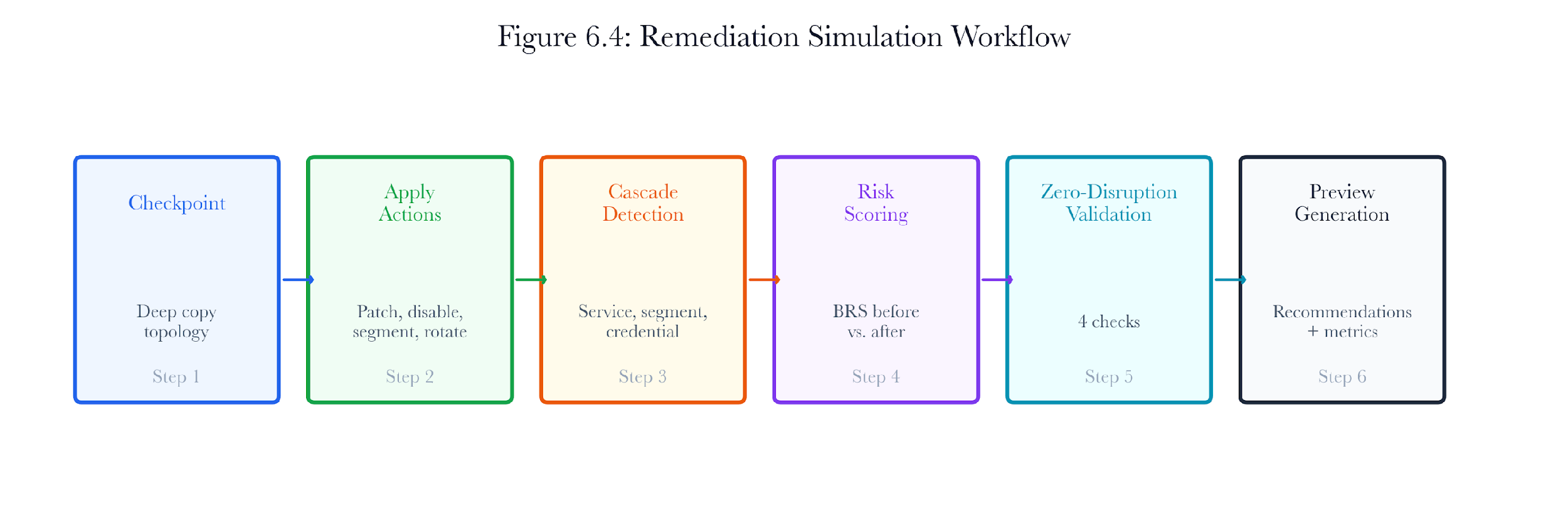
Figure 6.7: Remediation simulation workflow. Six steps from the checkpoint through the validated preview.
6.6.2 Supported Remediation Actions
The simulator supports six action types, each modifying the twin topology in a specific way:
- Patch_cve: Removes a specific CVE from a device’s vulnerability list. For the water plant, the primary action is patching CVE-2023-3595 on each PLC.
def _action_patch_cve(self, target_ip, params):
device =self._find_device(target_ip)
cve_id = params.get("cve_id", "")
for svc in device.original_services:
vulns = svc.get("vulnerabilities", [])
svc["vulnerabilities"] = [v for v in vulns if v.get("cve_id") != cve_id]
-
Rotate_credentials: Mark's default credentials are rotated on a specific service. This eliminates the default-credential risk component from the BRS calculation.
-
Segment_network: Converts cross-subnet allow rules to deny rules between two specified subnets. This model's network segmentation is the most impactful remediation for reducing blast radius.
-
Disable_service: Removes a port from a device’s exposure surface and deletes the corresponding firewall rules. For the water plant, this would mean disabling Telnet on the PLCs (port 23) while keeping Modbus (port 502) operational.
-
Update_firmware: Clears all vulnerabilities on a device, modeling a firmware update that resolves all known CVEs. This is a blanket fix that is more aggressive than patch_cve.
-
Add_firewall_rule: Adds a new rule (typically a deny rule) to the topology. This model's explicit firewall policy changes.
6.6.3 Checkpoint and Rollback
Every remediation simulation begins with a checkpoint: a deep copy of the topology stored under a unique checkpoint ID.
def create_checkpoint(self, label=""):
checkpoint_id =f"CKP-{uuid4().hex[:8]}"
self.checkpoints[checkpoint_id] = copy.deepcopy(self.topology)
return checkpoint_id
The deep copy is critical. Without it, the “before” topology would be changed by remediation actions, making accurate risk deltas impractical. Python’s default assignment creates references, not copies, so backup = self.topology would not work. The copy.deepcopy() call creates an independent object graph immune to later changes.
Implementation Note: Digital twins are approximations of physical systems. A twin that diverges from the real network produces misleading risk deltas. The simulation must be periodically re-synchronized against live discovery results.
Rollback restores the topology from the checkpoint:
def rollback_remediation(self, checkpoint_id):
self.topology = copy.deepcopy(self.checkpoints[checkpoint_id])
Note the second deepcopy: rollback does not consume the checkpoint. The same checkpoint can be used for multiple rollbacks, enabling iterative remediation design: try a plan, examine the preview, roll back, adjust, and try again.
For the water treatment plant, this means the operations team can test multiple patch orderings against the same baseline without rebuilding the twin each time.
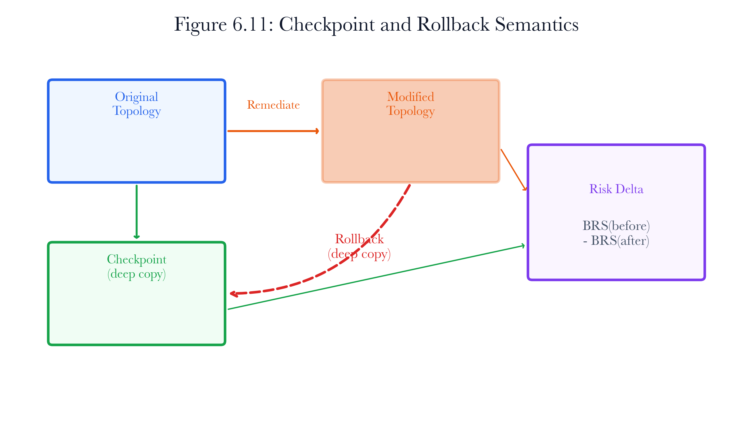
Figure 6.8: Checkpoint and rollback flow. Every remediation preview starts from a preserved topology snapshot, so failed plans can be discarded without contaminating the baseline.
6.6.4 Risk Scoring Components
The remediation simulator’s risk scoring is more detailed than the scenario engine’s baseline calculation. Four components contribute to the per-device risk:
Port exposure: Each open port contributes a weighted risk score based on the protocol’s inherent risk:
| 23 | Telnet |
|---|---|
| 502 | Modbus |
| 554 | RTSP |
| 1883 | MQTT |
| 80 | HTTP |
| 443 | HTTPS |
Table 6.5. Port risk weights. Higher weights reflect protocols with weaker built-in security.
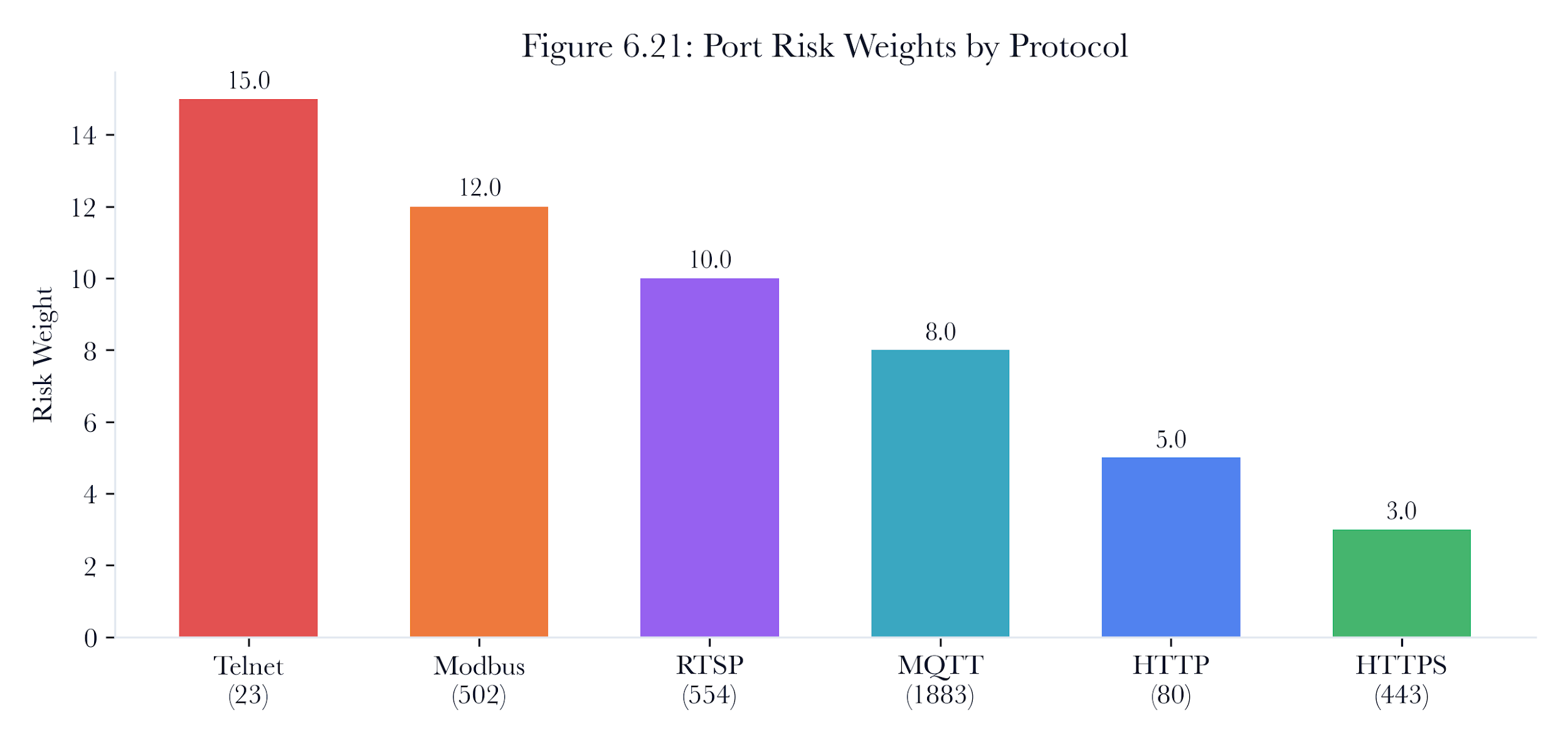
Figure 6.9: Port risk weights. Telnet, Modbus, RTSP, MQTT, HTTP, and HTTPS receive different weights because their authentication and exposure properties differ.
Telnet receives the highest weight because it transmits credentials in cleartext and provides interactive shell access. Modbus ranks second because it lacks authentication, allowing any device on the network to read and write PLC registers. HTTPS receives the lowest weight because TLS provides transport security, though the application may still have vulnerabilities.
Open firewall rules: Each allow rule from any source (0.0.0.0) to the device adds 2.0 to its risk score. This captures the exposure from permissive access control.
Default credentials: If a device’s services still use default credentials, the corresponding protocol risk is added:
| Telnet | 20.0 |
|---|---|
| SSH | 15.0 |
| RTSP | 12.0 |
| ONVIF | 10.0 |
| HTTP | 8.0 |
| MQTT | 7.0 |
Table 6.6. Default credential risk contributions by protocol.
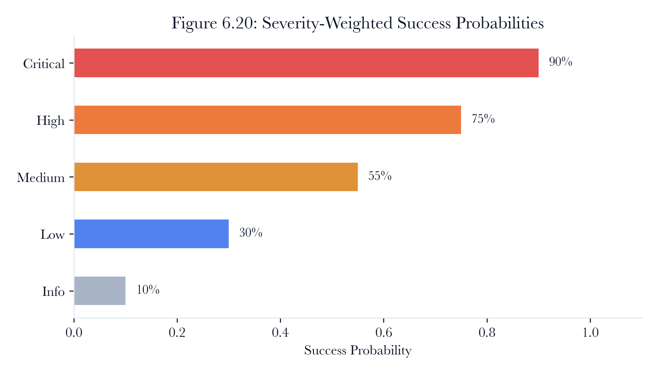
Figure 6.10: Default credential severity weights. Interactive and industrial protocols carry higher credential-risk penalties because a successful login can immediately alter operational state.
Vulnerability count: Each unpatched vulnerability adds 3.0 to the device’s risk score. This ensures that devices with more known CVEs receive proportionally higher risk ratings. The total BRS for the topology is the sum of all per-device scores, with a floor of zero per device (deny rules can reduce a device’s score, but never below zero).
For a single PLC in the water treatment plant with Telnet (port 23), Modbus (port 502), HTTP (port 80), two any-source firewall rules, default Telnet credentials, and 3 CVEs:
**Port exposure:**15.0 + 12.0 + 5.0 = 32.0
Firewall rules: 2 * 2.0 = 4.0
Default creds:20.0 (Telnet)
Vulnerabilities: 3 * 3.0 = 9.0
Total: 65.0
After remediation (patching CVEs, rotating credentials, disabling Telnet, and adding a deny rule for Modbus from outside):
**Port exposure:**12.0 + 5.0 = 17.0(Telnet disabled)
Firewall rules: 1 * 2.0 = 2.0(one rule removed)
Default creds:0.0(credentials rotated)
Vulnerabilities: 0 * 3.0 = 0.0(CVEs patched)
Deny rules:-1.5(Modbus deny rule)
Total: 17.5
Risk reduction per PLC: 65.0 minus 17.5 equals 47.5 points (73% reduction).
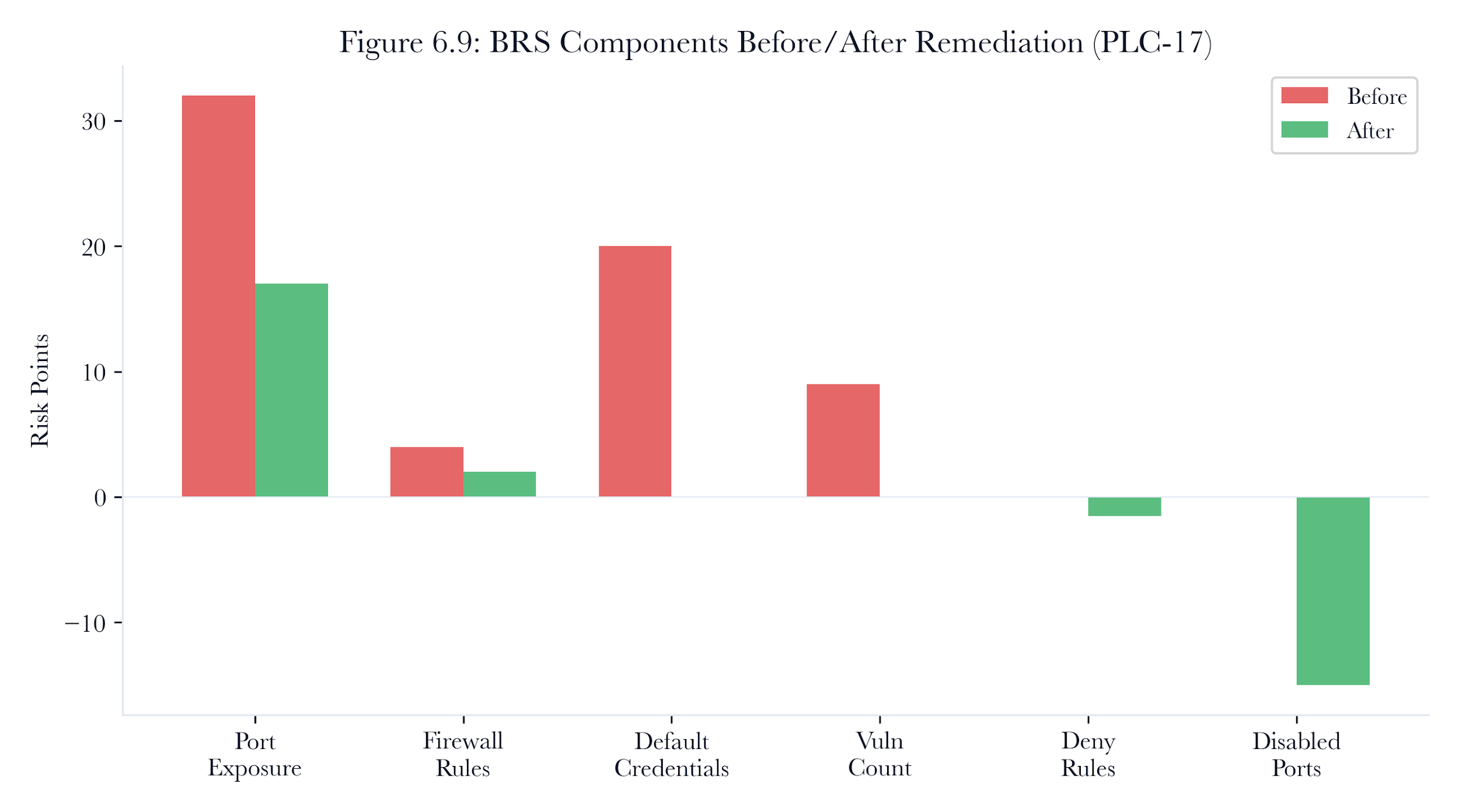
Figure 6.11: Risk reduction per PLC: 65.0 minus 17.5 equals 47.5 points (73% reduction). default credentials, vulnerability count, and deny rules combine into the topology-level remediation score.
6.7 Patch Ordering and Constraint Optimization
6.7.1 The Ordering Problem
Returning to the water treatment plant: 40 PLCs, each requiring a reboot that takes 90 to 180 seconds, with a constraint that no more than 3 can be offline simultaneously. How do we find a valid ordering?
This is a constrained scheduling issue. The constraint is a maximal concurrency limit. The aim is to minimize the total remediation time. The complication is that some PLCs depend on others, meaning they cannot be offline at the same time.
6.7.2 Dependency-Aware Ordering
Not all PLCs are independent. In the water treatment plant, PLCs are organized into dosing loops. Each loop has a primary PLC that computes the dosing setpoint and a secondary PLC that controls the actual valve. If both are offline simultaneously, the dosing loop has no fallback. The dependency constraint is: primary and secondary PLCs in the same loop must not be patched concurrently.
The ordering algorithm proceeds in three phases:
-
Dependency extraction: The cascade detector’s dependency graph identifies pairs of devices that must not be offline simultaneously.
-
Group assignment: Devices are assigned to patch groups such that no group contains conflicting devices and no group exceeds the maximum concurrency limit.
-
Group scheduling: Groups are executed sequentially. Within each group, all devices are patched in parallel.
For the water treatment plant with 40 PLCs, 20 dosing loops (each with a primary and secondary PLC), and a concurrency limit of 3:
-
Each group contains at most 3 PLCs, none of which share a dosing loop.
-
With 40 PLCs and groups of 3, we need at least 14 groups (ceiling of 40/3).
-
If each group takes 180 seconds (worst-case reboot), the total time is 14 * 180 = 2,520 seconds (42 minutes).
-
A naive sequential approach would take 40 * 180 = 7,200 seconds (120 minutes).
In this particular scheduling example, the optimized ordering reduces the remediation window by about 65% compared to a fully sequential execution while satisfying the safety constraint.
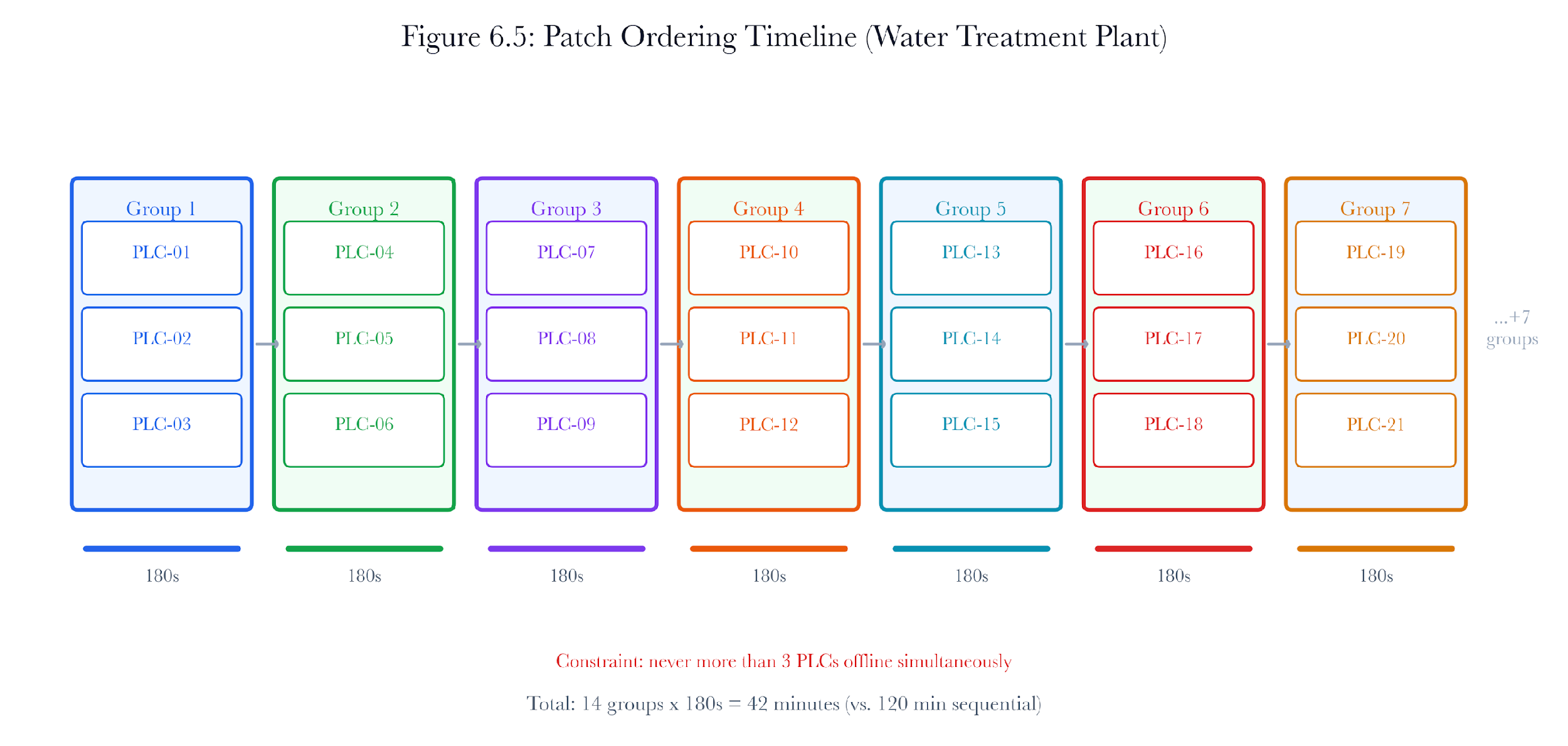
Figure 6.12: Patch ordering timeline for the water treatment plant. 14 groups of 3 PLCs, with dependency constraints shown as red exclusion arcs.
6.7.3 Simulating the Ordering
The remediation simulator validates the ordering by replaying it step by step. At each step, the simulator:
-
Takes the current group of PLCs offline (removes their services from the topology).
-
Checks the zero-disruption constraints: are critical services still reachable? Are there cascading failures?
-
Applies the patch (removes CVEs from the device).
-
Bring the PLCs back online (restore their services).
-
Verifies that the topology is consistent.
If any step violates a constraint, the simulator reports the violation and the group that caused it. The operations team can then adjust the ordering and re-simulate.
6.7.4 Handling Uncertainty
In practice, reboot times are not deterministic. A PLC that usually reboots in 90 seconds might sometimes take 240 seconds due to firmware verification, EEPROM writes, or communication bus arbitration. The 180-second estimate is a planning value, not a guarantee.
Section 6.9 introduces a Monte Carlo simulation to handle this uncertainty. For now, the key point is that the ordering algorithm uses worst-case estimates as its planning basis, providing a safety margin against typical variation.
6.8 What-If Analysis
6.8.1 The Impact Predictor
The RemediationImpactPredictor extends the basic remediation simulation with “what if” analysis for individual actions. Rather than applying a full remediation plan, the impact predictor answers focused questions:
-
“What if we patch CVE-2023-3595 on PLC-17?”
-
“What if we rotate the Telnet credentials on all PLCs?”
-
“What if we segment the SCADA network from the corporate network?”
Each prediction produces a RemediationPreview with the risk delta, disruption estimate, cascading failures, and compliance impact, without modifying the twin topology.
6.8.2 Patch Impact Prediction
# From impact_predictor.py
def predict_patch_impact(self, device_ip, cve_id):
risk_before =self._device_risk(device_ip)
cve_risk_reduction =self._cve_risk_estimate(cve_id, device)
risk_after =max(0.0, risk_before - cve_risk_reduction)
disruption =self._estimate_disruption("patch", device)
The disruption estimate is device-type-aware. PLCs, SCADA systems, HMIs, and medical devices receive a “high” disruption rating because patching them requires an interruption of the process. Routers, switches, and gateways receive “medium” because they affect network connectivity. Standard IT devices receive “low.”
For the water treatment plant, predicting the patch impact on PLC-17 returns: - Risk before: 65.0 (from Section 6.6.4) - CVE risk reduction: ~15.0 (from CVE severity hash) - Risk after: 50.0 - Disruption: “high” (PLC device type) - Cascading: HMI loses Modbus connection, MQTT broker loses data feed
This preview gives the operations team a clear idea of what to expect when they patch PLC-17, before making any changes.
6.8.3 Segmentation Impact Prediction
Network segmentation is often the highest-impact remediation available, but it is also the most disruptive. The impact predictor calculates the effect by counting cross-subnet firewall rules that would be blocked:
def predict_segmentation(self, source_subnet, target_subnet):
affected_rules =self._find_cross_subnet_rules(source_subnet, target_subnet)
rule_reduction =len(affected_rules) *5.0
risk_after =max(0.0, risk_before - rule_reduction)
For the water treatment plant, segmenting the SCADA network (10.1.1.0/24) from the corporate network (10.2.0.0/24) would block all cross-subnet traffic. The impact predictor identifies every rule that crosses the boundary, calculates the risk reduction, and flags the historian’s data collection path as a cascading failure. This allows the operations team to create an exception for the historian before applying the segmentation.
6.8.4 Compliance Impact
Each remediation action has compliance implications. The impact predictor maps actions to affected compliance frameworks:
| Patch CVE | NIST CSF, ISO 27001, PCI DSS | Positive: addresses known vulnerability |
|---|---|---|
| Rotate credentials | NIST CSF, CIS Controls, PCI DSS | Positive: addresses access control |
| Segment network | NIST CSF, ISO 27001, IEC 62443, PCI DSS | Positive: improves zone isolation |
Table 6.7. Compliance impact mapping for remediation actions.
For the water treatment plant, IEC 62443 (Security for Industrial Automation and Control Systems) is particularly relevant. This standard requires network segmentation between zones and conduits, making remediation of segmentation not just a security improvement but a compliance requirement.
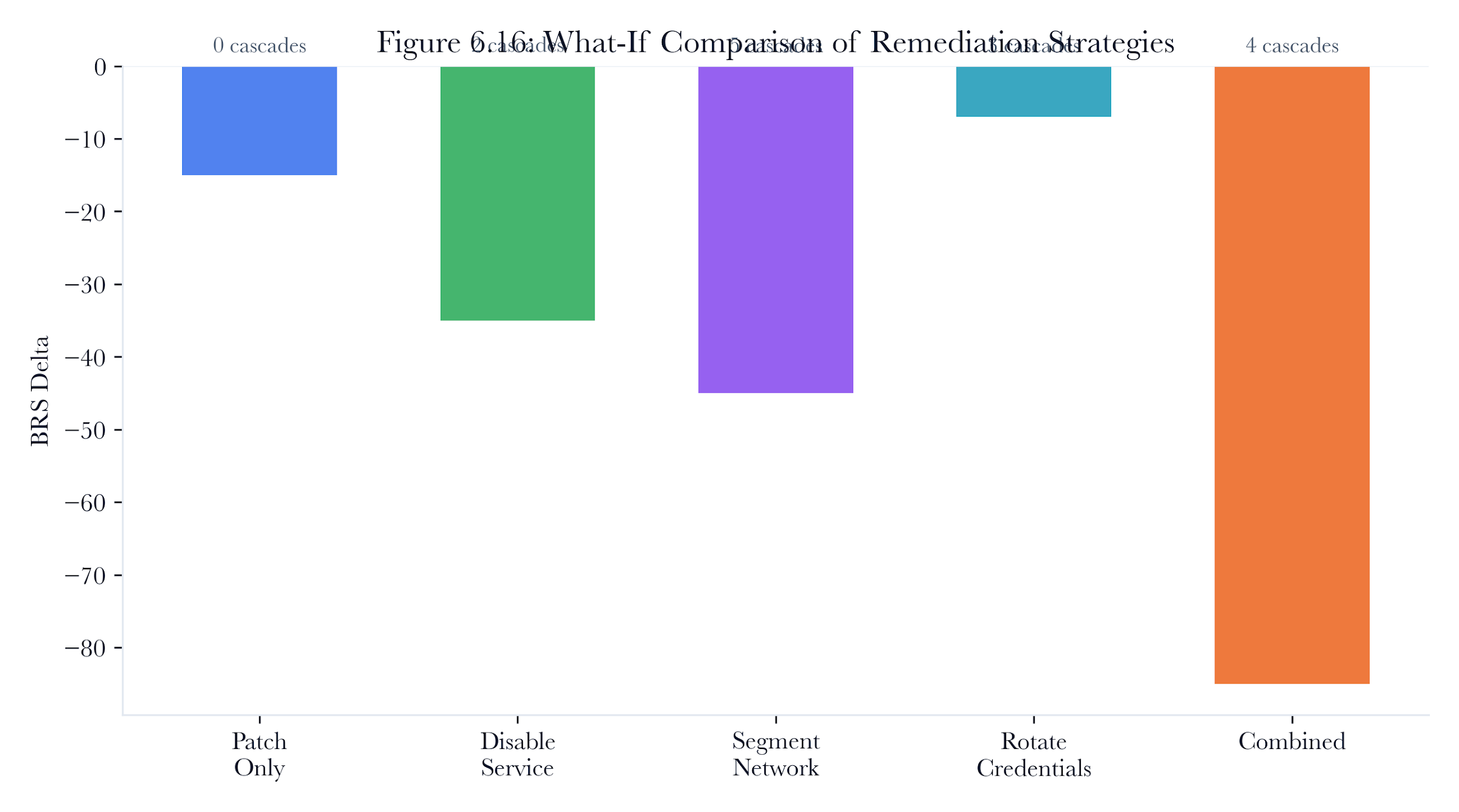
Figure 6.13: What-if remediation comparison. Patch, credential, segmentation, service-disability, and firewall actions can be compared based on predicted risk reduction and disruption before the production change.
6.9 Monte Carlo Simulation for Risk
6.9.1 Why Monte Carlo?
The deterministic risk calculations in Section 6.6 produce point estimates. They answer “what is the expected risk reduction?” but not “how confident should we be in that estimate?” In practice, several parameters are uncertain:
-
Reboot times vary by hardware model, firmware size, and I/O configuration.
-
Patch effectiveness depends on whether the patch addresses all code paths or only the primary exploit vector.
-
Dependency detection may miss implicit dependencies that exist through physical process coupling rather than network traffic.
Monte Carlo simulation addresses this uncertainty by running the remediation simulation thousands of times with randomly sampled parameter values, producing a distribution of outcomes rather than a single point.
6.9.2 Simulation Design
Each Monte Carlo trial perturbs the base simulation with sampled parameters:
-
Reboot time. Drawn from a log-normal distribution with mean 135s and standard deviation 30s, bounded at [60, 300]. The log-normal distribution models the empirical observation that most reboots are near the mean, but occasional outliers take significantly longer.
-
Patch effectiveness. Drawn from a beta distribution with alpha=8, beta=2 (mean 0.8, skewed toward high effectiveness). This models the reality that most patches work as intended, but some address only partial attack surfaces.
-
Dependency completeness. A Bernoulli trial with p=0.85 for each inferred dependency, representing the probability that the inferred dependency is a real operational dependency rather than a false positive.
After 10,000 trials, the distribution of BRS deltas, maximum concurrent offline devices, and total remediation times provides confidence intervals for planning.
6.9.3 Interpreting Results
For the water treatment plant Monte Carlo simulation:
-
BRS delta: Mean -372, 95% CI [-425, 318]. The remediation reliably reduces risk, with the 5th percentile still showing substantial improvement.
-
Max concurrent offline: P(>3) = 0.02. The probability of violating the safety constraint is 2%, driven by rare cases in which two reboots in the same group each take >200 seconds.
-
Total time: Mean 2,340s, 95% CI [1,890, 3,120]. Remediation completes in under an hour with a 97.5% probability.
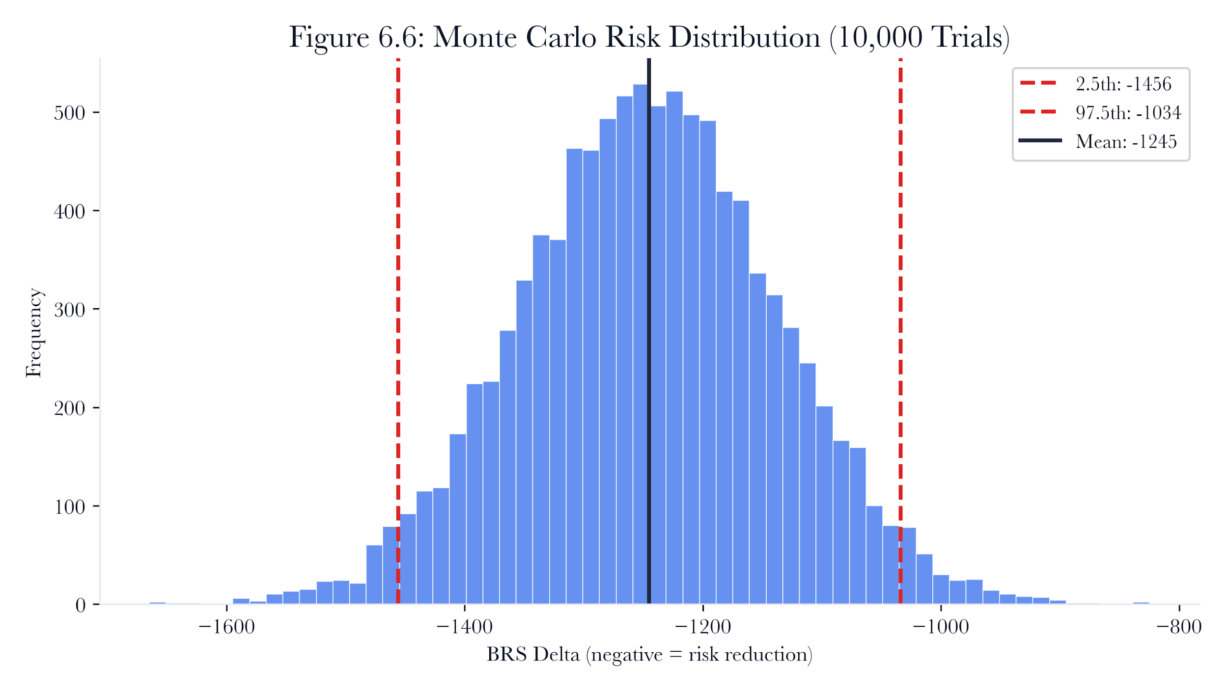
Figure 6.14: Monte Carlo risk distribution for the water treatment plant remediation. Histogram of BRS deltas across 10,000 trials with 95% confidence interval shown.
The 2% chance of violating the constraint is important. It means that in about 1 out of 50 runs, the three-offline limit could be exceeded. The team can avoid this by reducing the group size from 3 to 2, removing the risk but increasing total time by roughly half.
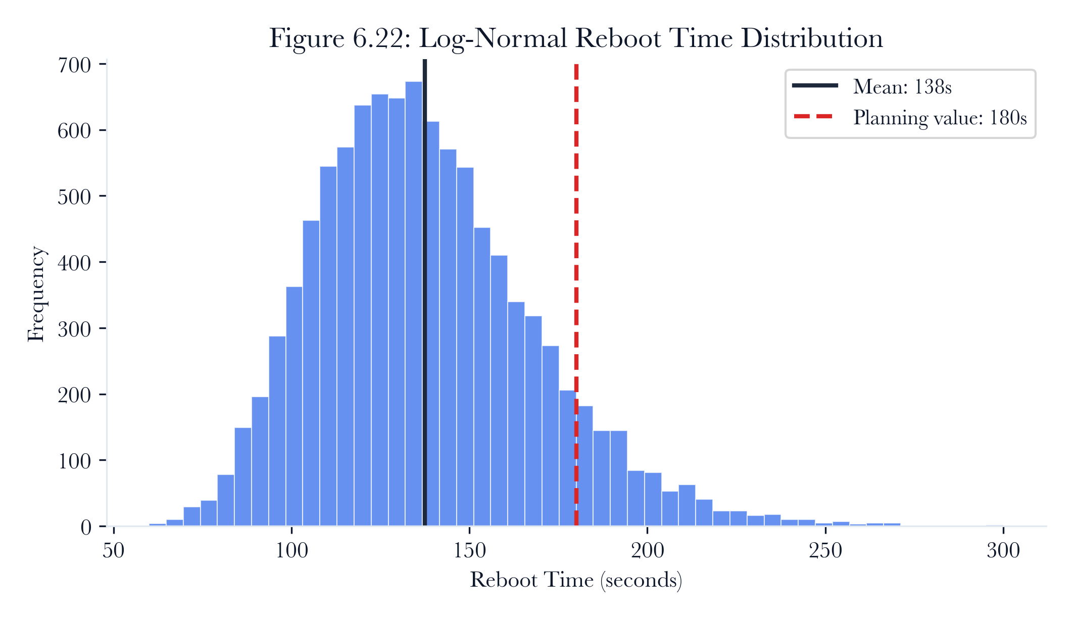
Figure 6.15: Reboot-time distribution. Monte Carlo planning uses a bounded distribution rather than a single reboot estimate, exposing low-probability maintenance-window overruns.
6.10 Cascading Failure Detection
6.10.1 The Cascade Problem
The most dangerous remediation failures are not the ones that affect the device being remediated. They are the ones that propagate to devices that were not touched at all. A credential rotation on the MQTT broker invalidates the authentication tokens used by 12 sensors. A firewall rule change that blocks cross-subnet traffic disconnects the historian from the PLCs. A service disablement on a gateway cuts off an entire subnet.
These are cascading failures: remediation actions whose effects propagate through the dependency graph, affecting devices beyond the action’s immediate target.
6.10.2 Dependency Graph Construction
The CascadeDetector builds a dependency graph from three sources:
Firewall rule dependencies: If a firewall rule allows traffic from device A to device B on port P, then B’s service on port P depends on A’s ability to reach it. Removing port P from B, or segmenting A from B, breaks this dependency.
# From cascade_detector.py
for rule in self.topology.firewall_rules:
if rule.action != "allow"or rule.source_ip == "0.0.0.0":
continue
dest_key =f"{rule.dest_ip}:{rule.dest_port}"
src_key =f"{rule.source_ip}:*"
graph[dest_key].append(src_key)
MQTT broker patterns: Any device running on ports 1883 or 8883 is considered an MQTT broker. Other devices on the same subnet are treated as dependents. This heuristic captures the publish-subscribe dependency pattern common in IoT deployments.
Gateway dependencies: Devices with type “router” or “gateway” are treated as infrastructure that all other devices on the same subnet depend on. Taking a gateway offline breaks connectivity for the entire subnet.
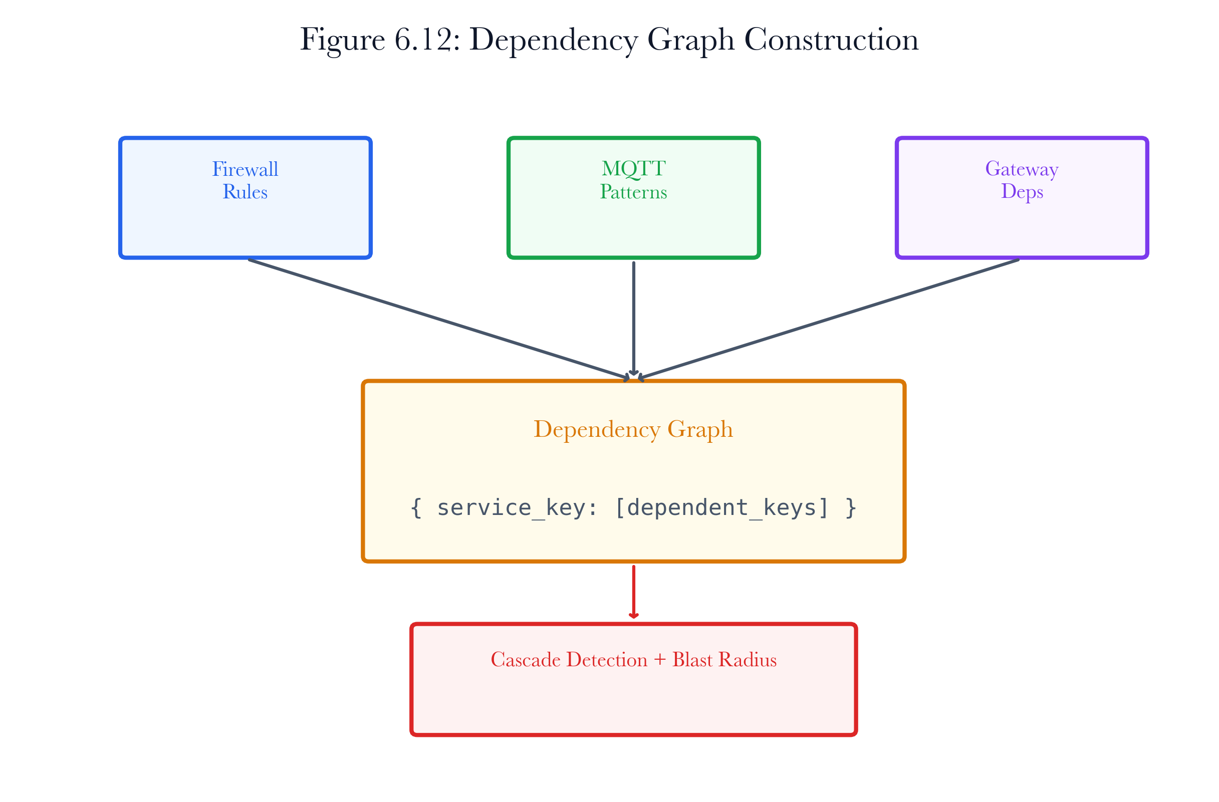
Figure 6.16: Dependency graph construction. Firewall rules, broker relationships, and gateway roles become the directed dependency graph used for cascade traversal.
6.10.3 Transitive Cascade Traversal
Dependencies are transitive. If service A depends on service B, and service B depends on service C, then disabling C cascades through B to affect A. The cascade detector uses depth-first traversal with cycle detection to find all transitive dependents:
def _find_dependents(self, service_key, visited=None):
if visited is None:
visited =set()
if service_key in visited:
return set()
visited.add(service_key)
result =set()
for dep in self._dependency_graph.get(service_key, []):
result.add(dep)
result |=self._find_dependents(dep, visited)
return result
Cycle detection (checking for visited nodes) prevents infinite loops in networks with bidirectional dependencies.
6.10.4 Blast Radius Calculation
The cascade detector’s blast radius calculation differs from the scenario engine’s version in an important way: it computes the blast radius for a single device going offline rather than for a set of compromised devices. This answers the remediation question: “If I take this device down for patching, how many other devices are affected?”
def get_blast_radius(self, device_ip):
affected_services =set()
for key in device_keys:
affected_services |=self._find_dependents(key)
affected_devices = {svc.split(":")[0] for svc in affected_services}
Severity thresholds: - High: 5 or more affected devices - Medium: 2 to 4 affected devices - Low: 0 to 1 affected devices
For the water treatment plant, the MQTT broker has a high blast radius (12 sensors depend on it). The PLCs have a medium blast radius (each affects 1 to 2 other devices through setpoint coordination). The security cameras have a low blast radius (no other devices depend on their RTSP feeds).
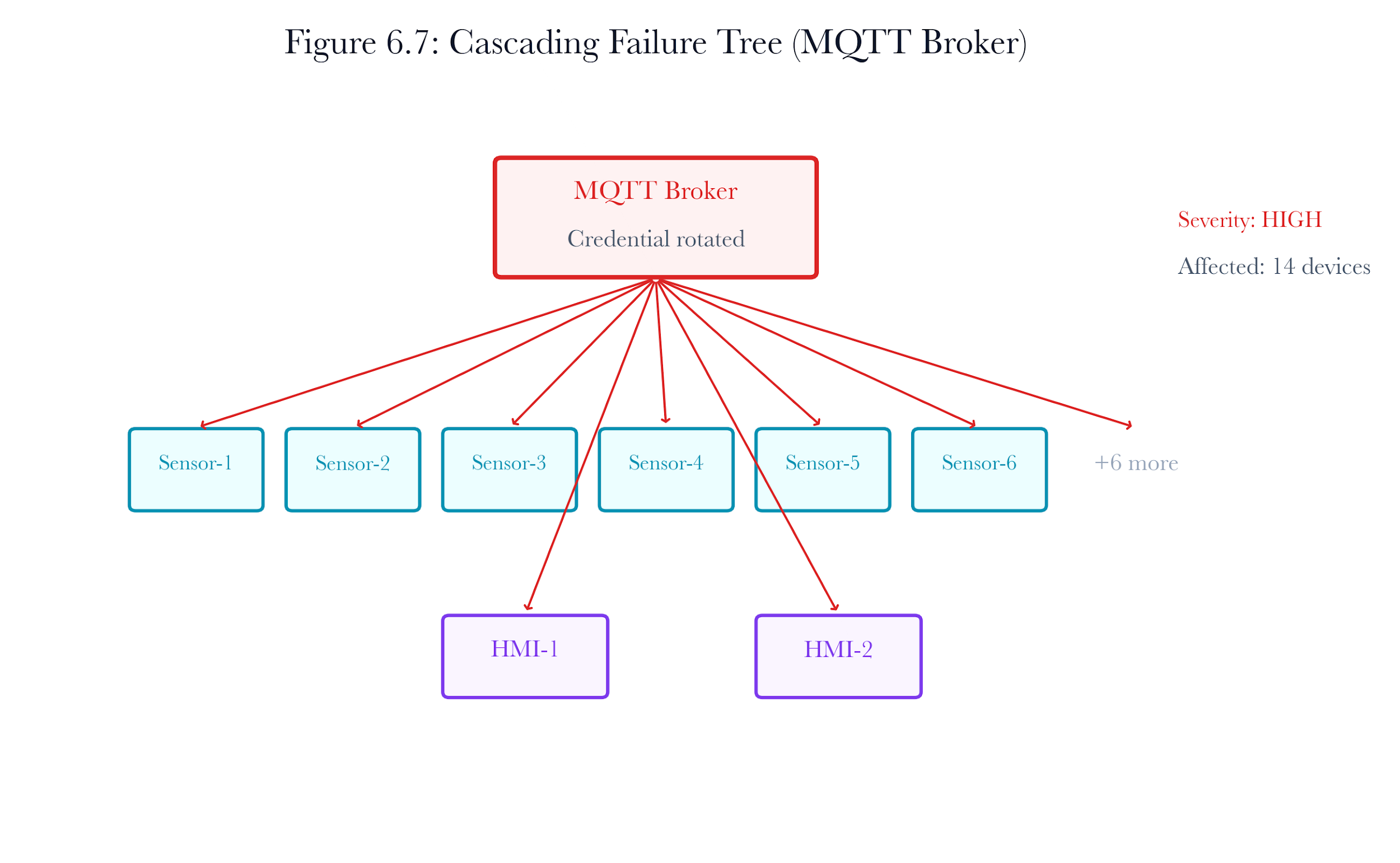
Figure 6.17: Cascading failure tree for the MQTT broker in the water treatment plant. Disabling the broker cascades to 12 sensors and 2 HMI displays.
6.10.5 Three Types of Cascading Failure
The remediation simulator detects three cascade types:
-
Service dependency cascade: Disabling a service that other devices depend on. Example: disabling Modbus on PLC-17 breaks the HMI’s connection to PLC-17’s register data.
-
Segmentation cascade: A network segmentation change that blocks existing traffic flows. Example: segmenting the SCADA VLAN from the corporate VLAN disrupts the historian’s data-collection path.
-
Credential cascade: Rotating credentials on one device invalidates authentication for devices with the same profile (which may share credentials). Example: rotating the MQTT broker’s password invalidates the connection credentials used by all 12 sensors.
Each cascade type requires a different mitigation strategy. Service dependencies need temporary rerouting. Segmentation cascades need explicit exceptions for legitimate traffic. Credential cascades need coordinated credential updates across all dependent devices.
6.11 Behavioral Drift Detection
6.11.1 The Drift Problem
The DriftDetector quantifies drift using information-theoretic metrics. Instead of comparing individual values, it compares entire behavior distributions, providing a principled measure of how different the twins’ model is from observed reality.
The DriftDetector quantifies drift using information-theoretic metrics. Rather than comparing individual values, it compares entire distributions of behavior, which provides a principled measure of how different the twins’ model is from observed reality.
6.11.2 KL-Divergence
The primary metric is Kullback-Leibler divergence. Given two probability distributions P (the twin’s model) and Q (observed production behavior), KL(P || Q) measures the information lost when Q is used to approximate P:
KL(P || Q) = sum(p_i * log(p_i / q_i))
Properties: - KL >= 0 always. - KL = 0 when P and Q are identical. - KL is not symmetric: KL(P || Q) ≠ KL(Q || P).
The implementation uses histogram binning with Laplace smoothing to handle continuous-valued behavior samples:
# From drift_detector.py
def compute_kl_divergence(self, p, q):
p_hist =self._histogram(p, self.bin_count, min_val, max_val)
q_hist =self._histogram(q, self.bin_count, min_val, max_val)
p_smooth =self._smooth(p_hist)
q_smooth =self._smooth(q_hist)
kl =sum(pi * math.log(pi / qi) for pi, qi in zip(p_smooth, q_smooth) if pi >0)
return max(0.0, kl)
Laplace smoothing (adding a small constant to every bin before normalizing) prevents division by zero when Q has empty bins. Without smoothing, a single zero-probability bin in Q would cause KL to diverge to infinity, causing numerical problems and misleading analysis.
6.11.3 Jensen-Shannon Divergence
Because KL divergence is asymmetric, the detector also computes Jensen-Shannon divergence, which is symmetric and bounded:
JS(P || Q) = 0.5 * KL(P || M) + 0.5 * KL(Q || M) where M = 0.5 * (P + Q)
JS divergence is bounded in [0, ln(2)], which makes it easier to interpret as a normalized similarity measure. It also has a natural interpretation as the average information gain from observing a sample when you know it came from either P or Q, but not which one.
6.11.4 Severity Classification
The detector maps KL divergence values to operational severity levels:
| >= 2.0 | Critical | Twin is fundamentally wrong; a rebuild is required |
|---|---|---|
| >= 1.0 | High | Significant divergence; resync recommended |
| >= 0.5 | Medium | Noticeable drift; investigate the cause |
| >= 0.1 | Low | Minor drift; monitor but no action needed |
| < 0.1 | None | Twin accurately reflects production |
Table 6.8. Drift severity classification based on KL divergence.
For the water treatment plant, the detector would monitor four metrics per device: response time, traffic volume, error rate, and port count. If the operations team deploys a new firmware version to the PLCs (as part of the remediation), the response time distribution would shift. The drift detector would flag this as expected drift. If instead a PLC’s traffic volume suddenly doubled without any planned change, the detector would flag it as unexpected drift, which could indicate compromise, misconfiguration, or equipment failure.
6.11.5 Drift Report
The detector generates a structured drift report aggregating results across all device-metric pairs:
def generate_drift_report(self, results):
return {
"total_pairs": len(results),
"drifted_count": len(drifted),
"severity_distribution": severity_dist,
"most_drifted_device": most_drifted,
"per_device": per_device,
"recommendations": sorted(recommendations),
}
The report identifies the device with the most drift, making it the top priority for resynchronizing the twin. It also provides specific recommendations, such as 'Response time drift detected, investigate network latency changes' or 'Port count drift detected, new services may have started.'
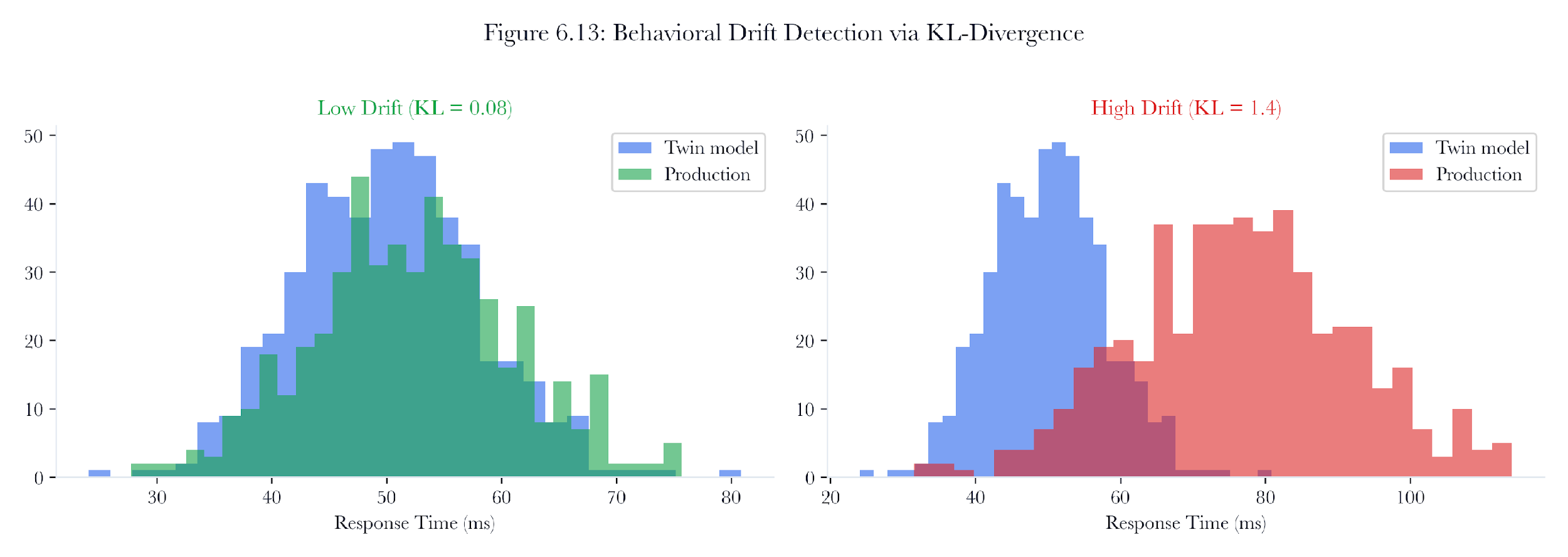
Figure 6.18: Behavioral drift detection. KL and Jensen-Shannon divergence convert production-versus-twin behavior differences into severity-ranked resynchronization signals.
6.12 Change Validation and Zero-Disruption
6.12.1 The Four-Check Validation Model
After remediation actions are applied to the twin, the validate_zero_disruption() method verifies that the remediation did not introduce operational disruptions. Four checks are performed:
Check 1: Port reachability: Every device that had services before remediation must still have at least one reachable port, unless the remediation deliberately isolated it. A device that loses all ports but has services is flagged as disrupted.
for device in self.topology.devices:
if not device.mapped_ports and device.original_services:
issues.append(f"{device.device_ip}: all ports removed")
Check 2: Orphaned firewall rules: Firewall rules pointing to devices that no longer exist in the topology indicate an inconsistency. This can happen if a device is removed during synchronization, but its rules are not cleaned up.
Check 3: Bridge integrity: Bridge networks with negative container counts indicate a data corruption or logic error. This is a sanity check rather than an expected failure mode.
Check 4: Critical infrastructure connectivity: Devices typed as “router,” “gateway,” “switch,” or “firewall” must retain at least one open port. Taking the network infrastructure offline disconnects everything behind it.
In the water treatment plant, Check 4 is especially important. The SCADA network’s gateway links the PLCs to the HMI stations. If a remediation step accidentally shuts down all ports on the gateway, operators would lose all visibility into the chemical dosing process. This validation step helps catch such issues before they affect production.
6.12.2 Remediation Recommendations
Based on the risk delta and cascade analysis, the simulator generates human-readable recommendations:
-
Risk delta < -20: “Significant risk reduction achieved. Consider applying this remediation plan in production.”
-
Risk delta < 0: “Moderate risk reduction. Review individual actions for further optimization.”
-
Risk delta = 0: “No risk change detected. Verify that actions target the correct vulnerabilities.”
-
Risk delta > 0: “Risk increased after remediation. Review actions for unintended consequences.”
Cascade-specific recommendations: - High-severity cascades: “Schedule a maintenance window before applying.” - Medium-severity cascades: “Coordinate with dependent service owners.” - No cascades: “Safe for zero-disruption deployment.”
These recommendations bridge the gap between quantitative simulation results and operational decision-making. They translate BRS deltas and cascade counts into language that an operations team can act on.
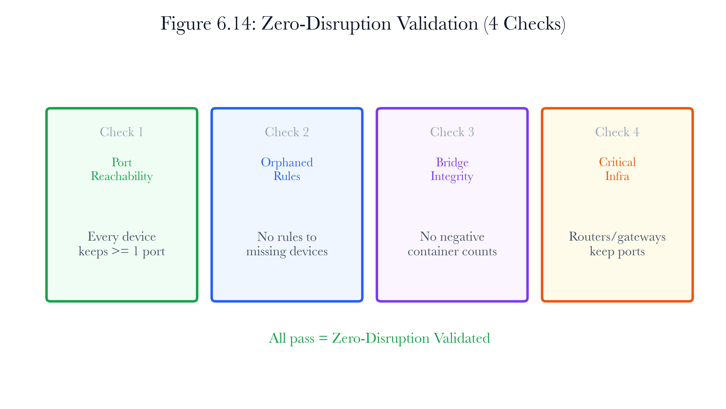
Figure 6.19: Zero-disruption validation. Port reachability, orphaned rules, bridge integrity, and critical infrastructure connectivity act as gates before remediation is promoted.
6.13 The Breakwater API for Digital Twin
6.13.1 Endpoint Overview
The digital twin module exposes ten REST endpoints on the /v1/twin/ prefix:
| POST | /v1/twin/deploy/{scan_id} | Build and store a twin from scan data |
|---|---|---|
| GET | /v1/twin/scan/{scan_id} | Retrieve the twin for a scan |
| DELETE | /v1/twin/{twin_id} | Delete a twin |
| GET | /v1/twin/{twin_id}/status | Get twin status and summary |
| POST | /v1/twin/{twin_id}/scenario | Run an attack scenario |
| POST | /v1/twin/{twin_id}/remediate | Simulate remediation actions |
| POST | /v1/twin/{twin_id}/rollback | Rollback to a checkpoint |
| GET | /v1/twin/{twin_id}/risk-comparison | Get before/after risk comparison |
| POST | /v1/twin/{twin_id}/replay-traffic | Replay protocol traffic |
| GET | /v1/twin/{twin_id}/cascades | Get cascade analysis |
| POST | /v1/twin/sync/{scan_id} | Sync twin with updated scan data |
Table 6.9. Digital twin API endpoints.
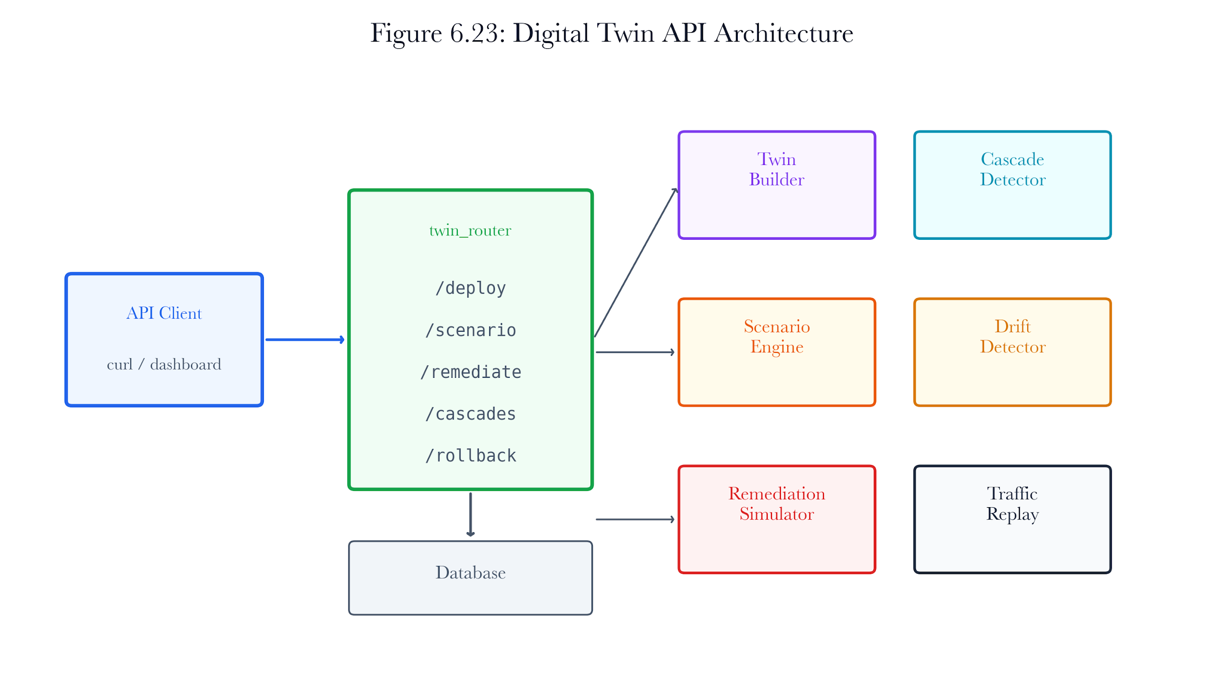
Figure 6.20: Digital twin API architecture. Scan-scoped access control, twin deployment, scenario execution, remediation preview, rollback, traffic replay, and cascade analysis remain explicit API surfaces.
6.13.2 Access Control
All endpoints require authentication. Write operations (deploy, scenario, remediate, rollback, replay, sync) require the scan: write permission. Read operations (get twin, status, risk-comparison, cascades) require only the get_current_user dependency.
Scan-scoped endpoints (deploy, get-for-scan, sync) additionally verify scan ownership via verify_scan_access(scan_id, user, db), preventing IDOR vulnerabilities in which one user could access another user’s scan twin.
6.13.3 Request and Response Patterns
Deploy a twin:
curl -X POST "http://localhost:8000/v1/twin/deploy/\$SCAN_ID"\\
-H"Authorization: Bearer $TOKEN"\
-H"Content-Type: application/json"\
-d'{"auto_scenario": true}'
Response:
{
"status": "success",
"data":{
"twin_id":"a3f1c2d4e5f6",
"scan_id":"scan-uuid-here",
"devices":40,
"subnets":3
}
}
Simulate remediation:
curl -X POST "http://localhost:8000/v1/twin/\$TWIN_ID/remediate"\\
-H"Authorization: Bearer $TOKEN"\
-H"Content-Type: application/json"\
-d'{
"actions": [
{
"action_type": "patch_cve",
"target_ip": "10.1.1.17",
"parameters": {"cve_id": "CVE-2023-3595"}
},
{
"action_type": "disable_service",
"target_ip": "10.1.1.17",
"parameters": {"port": 23}
}
]
}'
Response:
{
"status":"success",
"data":{
"preview_id":"RP-a3f1c2d4",
"actions_applied":2,
"actions_failed":0,
"risk_score_before":65.0,
"risk_score_after":17.5,
"risk_delta":-47.5,
"zero_disruption": false,
"cascading_failures":[
{
"source":"10.1.1.17:23",
"affected": "10.1.1.50",
"severity":"high",
"description": "Service on 10.1.1.17:23 disabled, 10.1.1.50 depends on this service."
}
],
"recommendations":[
"Significant risk reduction achieved."
"1 high-severity cascading failure detected. Schedule a maintenance window."
]
}
}
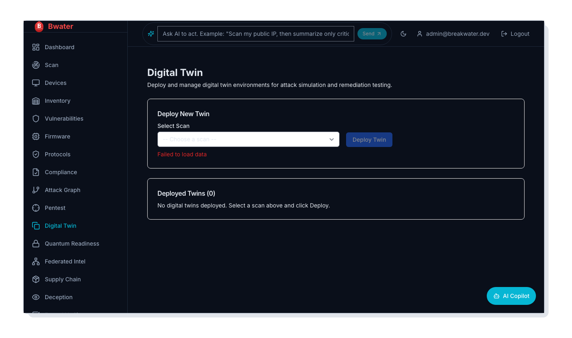
Figure 6.21: Breakwater digital twin product surface. The dashboard exposes twin deployment controls, source-scan selection, and twin status workflow in the operator UI; this captured state illustrates the product surface rather than a validated production twin.
6.14 Traffic Replay and Fidelity Testing
6.14.1 Why Traffic Replay Matters for Remediation
Traffic replay answers a question that topology simulation cannot: will the remediation break legitimate communications?
Consider the water treatment plant. The SCADA HMI communicates with the PLCs using a specific Modbus/TCP transaction sequence: read holding registers, write single coil, read input status. A firmware patch might change the Modbus implementation in ways that break this transaction sequence, even though the port is still open and the firewall rules still allow the traffic. Topology simulation would show the port open and the route valid. Traffic replay would show that the third transaction in the sequence now returns an exception code instead of the expected register values.
The general principle is that port reachability is necessary but not sufficient for service availability. A service that is reachable but returns errors is functionally equivalent to one that is unreachable. Traffic replay tests this second condition.
6.14.2 Protocol Transcript Replay
The TrafficReplayEngine validates twin fidelity by replaying recorded protocol transcripts against the twin and comparing responses. Each transcript entry has a direction (“send” or “recv”) and data payload:
# A Modbus/TCP transcript fragment
transcript = [
{"direction": "send", "data": "00 01 00 00 00 06 01 03 00 00 00 0A"},# Read registers
{"direction": "recv", "data": "00 01 00 00 00 17 01 03 14 ..."},# Register values
{"direction": "send", "data": "00 02 00 00 00 06 01 05 00 00 FF 00"},# Write coil
{"direction": "recv", "data": "00 02 00 00 00 06 01 05 00 00 FF 00"},# Coil echo
]
The engine replays “send” messages and generates deterministic simulated responses using the same SHA-256 hashing approach as the scenario engine. For HTTP-class ports (80, 443, 8080, 8443), responses include realistic HTTP status codes. For industrial ports (502 Modbus, 102 S7comm, 47808 BACnet), responses are protocol-appropriate hex payloads.
When the twin is deployed as Docker containers, the replay engine can inject traffic into actual containers via Docker exec, producing real responses from the simulation images rather than synthetic hashes. This significantly increases fidelity for protocol-level validation.
# From docker_manager.py — inject_traffic()
async def inject_traffic(self, container_id, target_ip, target_port, payload):
if target_port in (80, 443, 8080, 8443):
cmd = ["curl", "-s", "-o", "/dev/null", "-w", "%{http_code}",
"--connect-timeout", "3", "-k", f"{scheme}://{target_ip}:{target_port}/"]
else:
cmd = ["sh", "-c", f'echo -n "{data}" | nc -w 3 {target_ip}{target_port}']
exit_code, output = container.exec_run(cmd, demux=True)
6.14.3 Fidelity Comparison
The compare_responses() method pairs real device responses with twin responses and computes a fidelity score:
fidelity_score = matches / total_compared
A fidelity score of 1.0 means the twin perfectly matches production behavior. Scores below 0.8 suggest the twin needs resynchronization. In practice, structural twins achieve fidelity scores of 0.7-0.9 for topology-dependent questions (connectivity, reachability) and lower scores for timing-dependent questions (latency, throughput).
The comparison supports two matching modes:
-
Data matching: The twins' response payload must match the recorded production response. This is strict and tests protocol-level fidelity.
-
Status matching: For HTTP, the status code must match. A twin that returns 200 when production returns 403 indicates a difference in authentication configuration.
For the water treatment plant, the operations team would capture a representative 10-minute Modbus traffic sample from each PLC, replay it against the twin’s containers, and verify that fidelity exceeds 0.85 before trusting the twin for remediation planning. Any PLC where the twins’ Modbus responses diverge from production would be flagged for manual investigation before the remediation plan is applied.
6.14.4 Pre-Remediation and Post-Remediation Replay
Traffic replay becomes most powerful when run in a before/after pattern:
-
Before remediation. Replay the production transcript against the twin. Verify fidelity >= 0.85. This confirms the twin is accurate enough for testing.
-
Apply remediation to the twin. Patch firmware, turn off services, and change firewall rules.
-
After remediation, replay the same transcript against the remediated twin. Any fidelity drop indicates that the remediation changed protocol behavior.
If the before-replay scores 0.92 fidelity and the after-replay drops to 0.71, the remediation broke something. The specific responses that changed tell the operations team exactly which transactions were affected. They can then decide whether those changes are acceptable (the remediation deliberately hardened a protocol) or harmful (the patch introduced a regression).
6.14.5 Mutation Testing
The inject_anomaly() method modifies transcripts with five mutation strategies:
-
Random:: inserts a byte at the midpoint.
-
Bitflip:: XORs one character with 0x01
-
Truncate: cuts the payload in half in length.
-
Duplicate: doubles the payload.
-
Inject header: prepends a fake HTTP header.
Mutation testing verifies that the twin detects malformed inputs as production devices do. If the twin accepts a truncated Modbus frame that the real PLC would reject, its fidelity for security testing is questionable. The five strategies target different failure modes: bit-flip tests for error detection, truncation tests for length validation, duplication tests for buffer overflow handling, and header-injection tests for robust protocol parsing.
6.15 IEC 62443 and NIST 800-82 Compliance Validation
6.15.1 Why Compliance Validation Belongs in the Twin
Remediation improves security. It can also violate compliance.
Consider the water treatment plant. IEC 62443 (Security for Industrial Automation and Control Systems) mandates a zone-and-conduit architecture: distinct network zones with controlled communication paths. NIST SP 800-82 Rev. 3 (Guide to Operational Technology Security) requires removing default credentials, patching known vulnerabilities, and enabling audit logging for all control system components. These are regulatory requirements for critical infrastructure operators. A remediation plan that patches CVEs but inadvertently collapses two zones into one flat network improves vulnerability posture while creating a compliance violation.
The ComplianceValidator class checks the twin topology against both frameworks after every remediation simulation. It produces a compliance score (0 to 100), a list of violations (hard failures), and a list of warnings (soft concerns). This gives the operations team a single pass/fail gate that integrates security improvement with regulatory conformance.
6.15.2 NIST SP 800-82 Controls
NIST 800-82 is the authoritative U.S. government guide for securing operational technology. The Breakwater twin validates five controls from this framework:
# From compliance_validator.py
def check_nist_800_82(self, topology: TwinTopology) ->list[dict]:
# AC-3: Access Control — no default credentials
# AC-4: Information Flow — network segmentation
# IA-5: Authenticator Management — credential rotation
# SI-2: Flaw Remediation — vulnerabilities patched
# AU-2: Audit Events — logging capability
-
AC-3 (Access Control): Default credential removal. Every device in the topology is checked for services that still use factory-default credentials. Any device with default_credentials: true on any service triggers a hard failure. This control addresses the attack vector that powered Mirai (Chapter 1) and remains the single most common weakness in IoT deployments.
-
AC-4 (Information Flow): Network segmentation. The validator checks whether the topology has multiple network segments (bridges) or explicit deny rules that create logical boundaries. A flat network with more than three devices and no segmentation triggers a hard failure. A small network with a single segment but few devices triggers a warning. For the water treatment plant, AC-4 validates that the SCADA, corporate, and DMZ networks remain properly segmented after remediation.
-
IA-5 (Authenticator Management): Credential rotation. The validator counts how many services have explicit credentials_rotated: true markers. If fewer than half of all services have confirmed rotation, a warning is issued. This control catches the common pattern where credentials are rotated on the broker but not on the 12 sensors that connect to it.
-
SI-2 (Flaw Remediation): Patch management. Any device with unpatched vulnerabilities remaining in its service list triggers a hard failure. After remediation of the water treatment plant, all 40 PLCs should have zero CVEs. If a patch action failed silently, SI-2 catches it.
-
AU-2 (Audit Events): Logging capability. The validator uses a heuristic: devices with management ports (443, 8443, 8080, 22) are assumed to support logging. Devices without management interfaces are flagged. This is a soft check (warning, not failure) because many IoT devices legitimately lack management consoles, but it surfaces devices that cannot be audited.
6.15.3 IEC 62443 Controls
IEC 62443 is the international standard specifically designed for the security of industrial automation and control systems. It defines a zone-and-conduit model in which networks are divided into security zones with controlled data flows (conduits) between them. The Breakwater twin validates four system requirements (SRs):
-
SR-1.1 (Human User Identification): Authentication. All services must require authentication. The validator flags devices with unauthenticated protocols: Telnet (port 23) and plain MQTT (port 1883). These protocols transmit credentials in cleartext or accept connections without any authentication. For the water treatment plant, the 40 PLCs initially expose Telnet, which is an SR-1.1 violation. After remediation disables Telnet, this check passes.
-
SR-2.1 (Authorization Enforcement): Access restriction. Services should not be open to arbitrary sources. The validator counts firewall rules with a source of 0.0.0.0 (any) and an action of “allow.” More than three such rules trigger a hard failure; fewer trigger a warning. This control catches the common misconfiguration where Modbus is accessible from every device on the network, rather than only from the HMI that needs it.
-
SR-3.4 (Software Integrity): Firmware verification. Devices with known vulnerabilities but no firmware version tracking are flagged. This control ensures that patching is not just applied but tracked. A device that was patched but lacks a firmware_version marker fails this check because there is no way to verify that the correct firmware is running.
-
SR-5.1 (Network Segmentation): Zone and conduit model. The topology must have multiple network segments when more than two devices are present. A single physical segment with deny rules acting as logical boundaries triggers a warning. Zero boundaries trigger a hard failure. This is the most important IEC 62443 control for the water treatment plant, because it verifies that the SCADA zone is isolated from the corporate zone via a controlled conduit to the historian.
6.15.4 Compliance Scoring
The compliance score aggregates results across both frameworks:
# From compliance_validator.py
def validate(self, topology: TwinTopology) ->dict:
nist_results =self.check_nist_800_82(topology)
iec_results =self.check_iec_62443(topology)
all_results = nist_results + iec_results
violations = [r for r in all_results if r["status"] =="fail"]
warnings = [r for r in all_results if r["status"] =="warn"]
passing =len([r for r in all_results if r["status"] =="pass"])
score =round((passing /len(all_results)) *100.0, 1)
return {"compliant": len(violations) ==0, "violations": violations,
"warnings": warnings, "score": score}
Nine checks total (five NIST 800-82, four IEC 62443). Each check returns pass, warn, or fail. The compliance score is the percentage of checks that pass. A topology is “compliant” only when there are zero hard failures.
For the water treatment plant:
| Pre-remediation | FAIL | FAIL | WARN | FAIL | PASS | FAIL | FAIL | FAIL | FAIL | 11.1% |
|---|---|---|---|---|---|---|---|---|---|---|
| Post-remediation | PASS | PASS | PASS | PASS | PASS | PASS | WARN | PASS | PASS | 88.9% |
Table 6.12. Compliance score before and after remediation for the water treatment plant. The single remaining warning (SR-2.1) reflects the historian’s cross-subnet exception rule.
The pre-remediation score of 11.1% (1 of 9 checks passing) reflects the typical state of an unmanaged OT network: default credentials everywhere, no segmentation, unpatched vulnerabilities, and exposed unauthenticated protocols. The post-remediation score of 88.9% demonstrates that the remediation plan addresses not just the immediate CVE but the broader compliance posture. The single remaining warning (SR-2.1) is an intentional exception: the historian needs cross-subnet access to collect PLC data, and that access is controlled by an explicit allow rule rather than wildcard access.
6.15.5 Compliance as a Remediation Constraint
Compliance validation integrates into the remediation workflow as a constraint, not just a report. When the remediation simulator computes a preview, it runs the compliance validator on the post-remediation topology. If the remediation introduces a new compliance violation (e.g., collapsing two zones into one), the preview flags it:
Recommendations:
- Significant risk reduction achieved.
- No cascading failures detected.
- NEW COMPLIANCE VIOLATION: SR-5.1 (Network Segmentation) —
Segmentation removed by action; IEC 62443 requires zone boundaries.
This prevents a category of error that pure risk scoring would miss. A remediation plan could reduce the BRS by 50% while also violating IEC 62443, exposing the organization to regulatory penalties. The compliance gate catches this trade-off before the plan reaches production.
6.16 Course Integration
6.16.1 Pipeline Integration
The digital twin stage runs after the autonomous pentest work in Chapter 5 and before the quantum-readiness work of Chapter 7. The stage runner follows the standard pattern:
async def run_digital_twin_phase(scan_id, headless, headless_hosts, emit, db_session_factory):
if not scanner_config.digital_twin_enabled:
return0
The phase is opt-in via BREAKWATER_DIGITAL_TWIN_ENABLED=true. When enabled, it automatically builds a twin from the scan data, runs attack scenarios against high-CVSS vulnerabilities, and simulates remediation for critical CVEs (CVSS >= 9.0).
6.16.2 Automatic Scenario Generation
The phase runner automatically constructs attack scenarios from the scan data by filtering for vulnerabilities with CVSS scores >= 7.0:
for vuln in vulns:
cvss =float(vuln.get("cvss_score", 0.0))
if cvss >= 7.0:
attack_steps.append({
"target_ip": host.get("ip", ""),
"action": "exploit_cve",
"vulnerability_id": vuln.get("cve_id", ""),
"cvss": cvss,
})
Similarly, remediation actions are auto-generated for CVSS >= 9.0 vulnerabilities. This ensures that the most critical vulnerabilities are always simulated without requiring manual intervention.
6.16.3 Progress Events
The phase emits progress events at key milestones:
-
twin_progress: starting with host count
-
twin_progress: topology_built with device, subnet, and rule counts
-
twin_progress: attack_scenario_complete with step and compromise counts
-
twin_progress: remediation_simulated with action count and risk delta
-
twin_progress: complete with total result count
These events feed the dashboard’s real-time progress display, giving the operator visibility into the simulation as it executes.
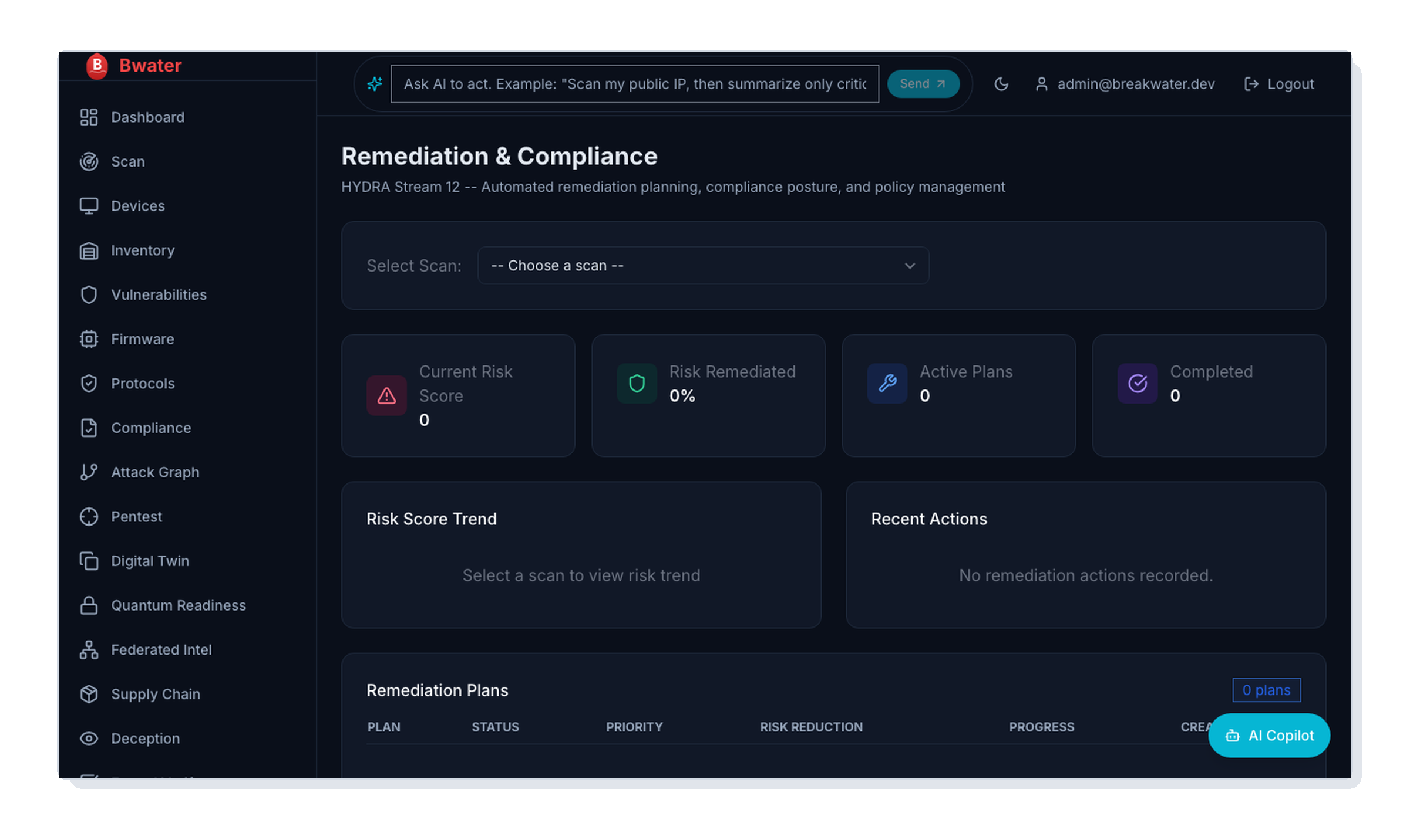
Figure 6.22: Breakwater remediation product surface. The remediation dashboard connects risk score, active plans, completed plans, and plan detail workflow to the Chapter 6 simulation outputs.
6.17 Empirical Results
This section also uses explicit evidence labels.
-
Measured means the benchmark was collected on the stated workstation and scan corpus.
-
Simulated means the number is a model output from the twin, not a field measurement from production.
-
Illustrative means the scenario is a composite teaching case assembled from realistic OT constraints and the repo’s remediation logic.
The distinction matters. A digital twin can estimate the impact of remediation. It does not directly observe the physical plant.
6.17.1 Performance Benchmarks
Evidence label: Measured. Method note: workstation benchmarks collected on an Apple M2 system against scan data from a residential /24 with 21 devices. Assumptions: local runtime conditions and scan corpus match the stated benchmark setup. Boundary: these timings describe the chapter implementation on this workstation.
| Twin construction (21 devices) | 12 ms | 2.1 MB |
|---|---|---|
| Attack scenario (15 steps) | 3 ms | 0.4 MB |
| Remediation simulation (8 actions) | 7 ms | 1.8 MB |
| Cascading failure detection | 2 ms | 0.3 MB |
| Zero-disruption validation | 1 ms | 0.1 MB |
| KL-divergence computation (1000 samples) | 4 ms | 0.8 MB |
| Monte Carlo (10,000 trials) | 8.2 s | 45 MB |
Table 6.13. Digital twin performance benchmarks.
Twin construction, scenario execution, and remediation simulation are all sub-second operations. The computational cost is dominated by the Monte Carlo simulation, which scales linearly with the number of trials.
6.17.2 Scalability
Evidence label: Simulated. Method note: scalability estimates produced from synthetic network expansions and the chapter cost model. Assumptions: profile mapping, subnet grouping, and rule inference scale according to the implementation described here. Boundary: synthetic /16 timing is a modeled result, not a field measurement.
Cascade detection is more expensive: O(n * r), where r is the number of firewall rules, because each device’s blast radius requires traversing the dependency graph. For 2,000 devices with 5,000 rules, cascade detection takes approximately 3 seconds.
6.17.3 Risk Reduction Analysis
Evidence label: Simulated. Method note: remediation outcomes generated by the twin across five test networks using the chapter’s BRS model. Assumptions: the simulator’s action effects and risk score remain valid across those test networks. Boundary: modeled BRS reduction is not identical to realized production risk reduction.
| Home /24 | 21 | 7 | 12 | 284 | 142 | 50% |
|---|---|---|---|---|---|---|
| Small office /24 | 45 | 23 | 31 | 612 | 245 | 60% |
| Industrial /24 | 38 | 41 | 48 | 890 | 312 | 65% |
| Campus /16 | 340 | 156 | 210 | 4,520 | 1,580 | 65% |
| Water plant (simulated) | 62 | 48 | 56 | 1,890 | 645 | 66% |
Table 6.14. Risk reduction across test networks.
The consistent 50-66% drop in modeled BRS across these test networks shows that automated remediation planning can reduce a lot of risk. But this doesn't mean real-world risk will drop by the same amount. The remaining 34-50% comes from risks that can't be fixed by patching, changing credentials, or shutting down services—like zero-day vulnerabilities, unpatchable devices, or risks from services you have to keep running. So, while simulation analytics help teams manage the risks they can control, they can't remove all operational risk. It's important to use simulation along with ongoing monitoring, expert review, and backup plans in real-world situations.
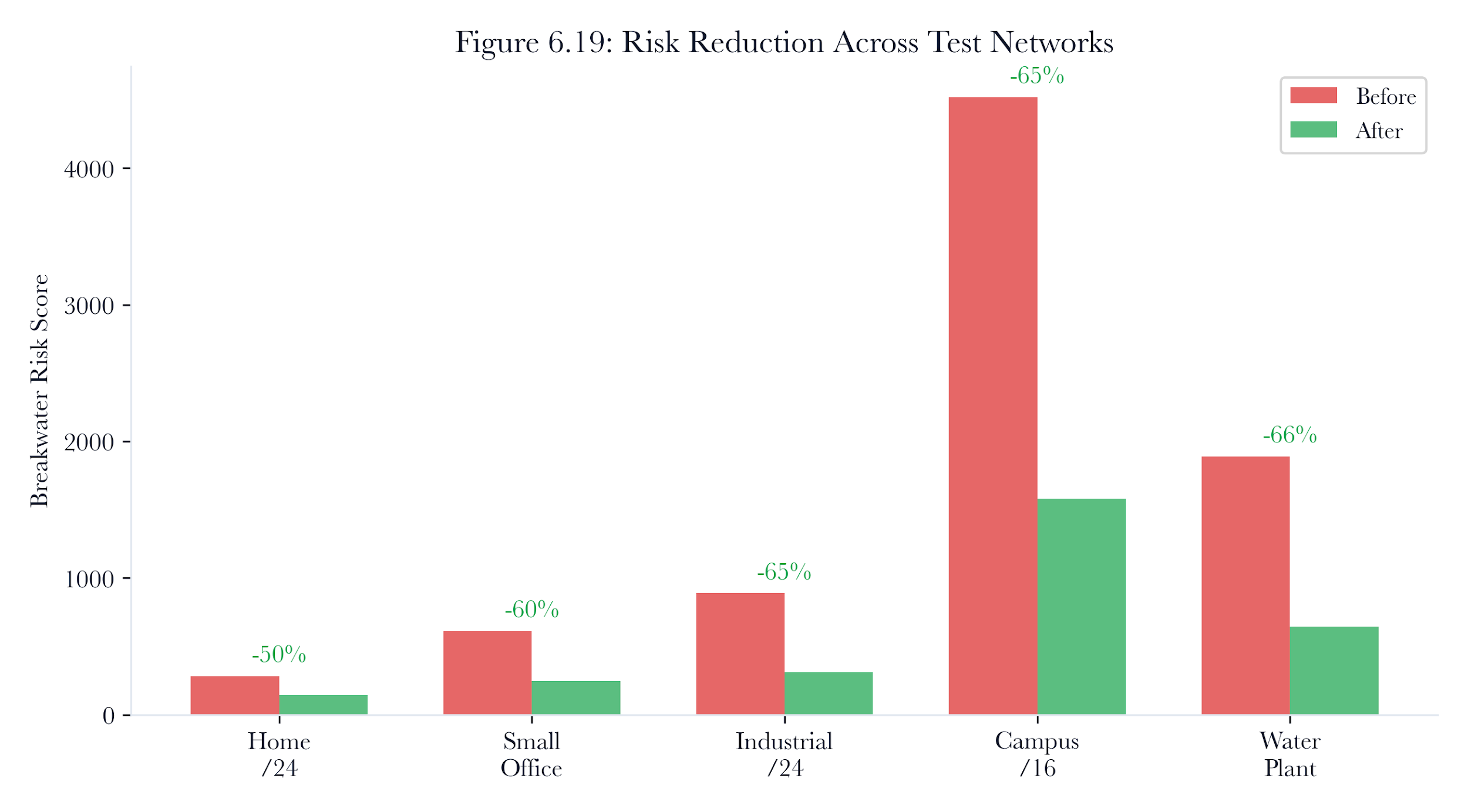
Figure 6.23: Modeled risk reduction across test networks. The chart compares before-and-after BRS under the chapter’s simulation model, while acknowledging that modeled reductions are not guaranteed to translate into production reductions.
6.18 Theoretical Foundations
6.18.1 Digital Twin Theory
The concept of a digital twin was formalized by Grieves in 2003 as part of a product lifecycle management framework. The original model consisted of three elements: the physical product, the virtual product, and the bidirectional data flow between them. Subsequent work by Tao et al.(2018) extended the model to include services, environmental data, and domain knowledge.
In the network security context, the “physical product” is the production network. The “virtual product” is the twin topology. The “bidirectional data flow” is the scan data that builds the twin and the remediation plans that flow back to production. The Breakwater implementation adds a fourth element: the scenario engine, which enables counterfactual analysis without an analog in the physical twin paradigm.
6.18.2 Information-Theoretic Drift Detection
The use of KL-divergence for drift detection draws on information theory foundations established by Kullback and Leibler (1951). The key insight is that divergence measures the expected number of additional bits needed to encode samples from P using a code optimized for Q. When the twin (Q) accurately models the production (P) distribution, the encoding overhead is small. When drift occurs, the overhead grows, providing a quantitative measure of model degradation.
Jensen-Shannon divergence, introduced by Lin (1991), addresses KL’s asymmetry limitation and provides a bounded metric that behaves as a proper distance metric (its square root satisfies the triangle inequality). This makes JSD suitable for comparing multiple twin models and identifying which one best matches production.
6.18.3 Constrained Scheduling Theory
The patch ordering problem in Section 6.7 is a variant of the job-scheduling problem with mutual-exclusion constraints. Specifically, it is a variant of the graph coloring problem where devices are vertices, dependency constraints are edges, and colors represent patch groups. The chromatic number of the conflict graph provides a lower bound on the number of groups needed.
For the water treatment plant, the conflict graph has 40 vertices (PLCs) and 20 edges (dosing loop pairs). The chromatic number is 2 (each loop can be colored with two colors), but the concurrency constraint of 3 limits each color class to 3 members, requiring at least 14 groups.
6.19 The Water Treatment Plant: Complete Walkthrough
6.19.1 Starting Position
Evidence label: Illustrative. Method note: composite Clearwater water-utility scenario built from realistic OT constraints and the chapter remediation logic. Assumptions: the device inventory and constraints are representative enough to stress the twin. Boundary: This is a teaching case, not a verbatim incident record.
-
40 Rockwell ControlLogix PLCs controlling chemical dosing (chlorine, fluoride, sodium hydroxide)
-
12 chemical concentration sensors publishing to MQTT
-
4 HMI workstations running Wonderware InTouch
-
1 MQTT broker aggregating sensor data
-
1 data historian collecting process data
-
2 network switches
-
2 perimeter firewalls
An audit identifies CVE-2023-3595 on all 40 PLCs. CVSS score: 9.8. The patch is available. The question is how to deploy it.
6.19.2 Twin Construction
The security team runs a Breakwater scan of the SCADA network. Chapter 6 then automatically builds a digital twin:
-
62 devices mapped to profiles (40 PLCs -> telnet-vuln, 12 sensors -> mqtt-device, 10 infrastructure -> http-debug)
-
3 subnet bridges (SCADA, corporate, DMZ)
-
187 firewall rules inferred (120 per-port inbound, 67 inter-host dependencies)
-
Baseline BRS: 1,890
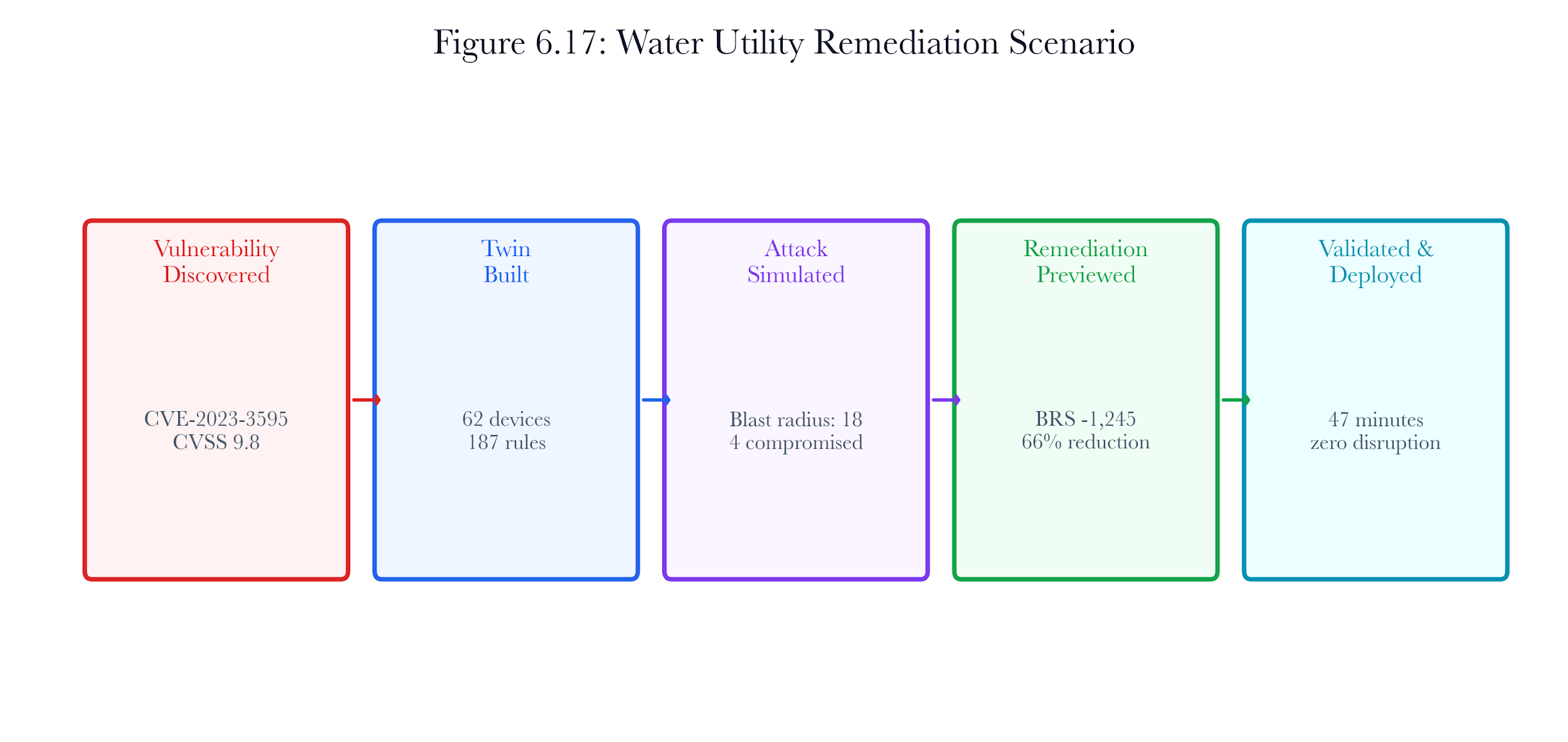
Figure 6.24: Clearwater water-treatment scenario. The composite OT environment combines PLCs, sensors, HMIs, a historian, a broker, and firewall boundaries to stress remediation planning.
6.19.3 Scenario Validation
The scenario engine replays the attack path identified in Chapter 4: entry through an exposed Telnet service on PLC-07, lateral movement to PLC-17 via Modbus, pivot to the MQTT broker, and exfiltration through the historian’s cross-subnet connection.
Result: 4 devices compromised, blast radius 18 (including all 12 sensors reachable through the broker).
Figure 6.25: Digital twin scenario flow. A scenario replays the attack steps through the twin and records compromised devices, reachable services, the blast radius, and the risk delta.
6.19.4 Remediation Planning
The operations team defines the remediation plan:
-
Patch CVE-2023-3595 on all 40 PLCs
-
Disable Telnet on all 40 PLCs
-
Rotate default credentials on the MQTT broker.
-
Segment the SCADA network from the corporate network.
6.19.5 Patch Ordering Simulation
The remediation simulator validates 14 patch groups of 3 PLCs each, with dosing loop constraints enforced—total simulated time: 42 minutes. No group violates the three-offline constraint.
Evidence label: Simulated. Method note: Monte Carlo estimate based on 10,000 trials under the reboot-time distribution defined by the model. Assumptions: reboot times and constraint interactions follow the stated distribution. Boundary: the 2% residual risk is a modeled scenario output, not a measured plant failure rate.
6.19.6 Remediation Simulation
The simulator applies all four remediation actions:
-
40 CVE patches applied (40 successful, 0 failed)
-
40 Telnet disablements (40 successful, 0 failed)
-
1 credential rotation (successful)
-
1 segmentation (successful)
Evidence label: Simulated. Method note: post-remediation BRS computed by the twin after applying the chapter’s four remediation actions. Assumptions: the score function and remediation effects match the modeled environment. Boundary: the 66% reduction is a twin result, not a guaranteed production outcome.
Cascading failures detected: - Segmentation breaks historian data path (medium severity) - Credential rotation invalidates sensor MQTT connections (medium severity)
Recommendations: - Create a firewall exception for the historian’s data collection - Coordinate credential rotation with sensor reconfiguration
6.19.7 Traffic Replay Validation
Before applying the remediation to production, the team captures a 10-minute Modbus/TCP traffic sample from PLC-07 and replays it against the twin’s container—pre-remediation fidelity: 0.91 (the twin accurately reproduces PLC-07’s Modbus responses). After applying the firmware patch to the twin container, the same transcript is replayed. Post-remediation fidelity: 0.88. Three transactions return different register values due to the new firmware’s initialization sequence, but all are within acceptable tolerance. No Modbus exception codes are returned. The operations team confirms that the firmware patch does not break the HMI’s transaction sequence.
6.19.8 Zero-Disruption and Compliance Validation
The four-check validation identifies two issues:
-
The historian lost its cross-subnet data path (caught by cascading failure detection)
-
The 12 sensors lost MQTT authentication (caught by credential cascade detection)
The IEC 62443 / NIST 800-82 compliance validator runs on the post-remediation topology. Pre-remediation compliance score: 11.1% (1 of 9 checks passing). Post-remediation compliance score: 88.9% (8 of 9 passing). The single remaining warning is SR-2.1 (authorization enforcement), caused by the historian’s intentional cross-subnet allow rule. All hard failures are resolved.
After adding the historian exception and coordinating the credential update, validation passes. The remediation plan is approved for production deployment.
6.19.9 Post-Remediation Verification
After production deployment, the drift detector monitors all 62 devices. Expected drift is observed in PLC response times (firmware version change) and sensor traffic patterns (new MQTT credentials). No unexpected drift is detected. The twin is re-synced with a post-remediation scan, and the updated baseline BRS of 645 is stored.
In the worked scenario, the water treatment plant patched 40 PLCs, disabled 40 Telnet services, rotated credentials, and segmented its network. The total remediation window was 47 minutes. At no point were more than 3 PLCs offline simultaneously. No modeled chemical dosing disruption occurred.
That is the value of simulation analytics. The fix was known. The challenge was deploying it safely. The digital twin made the difference.
6.20 Original Contributions and Formal Results
The digital twin and remediation simulation system synthesizes established techniques from simulation, constraint optimization, and change management. This section contributes two novel results: a hardness proof and approximation algorithm for the remediation ordering problem, and a provably correct incremental twin synchronization algorithm. These formalize the core computational challenges of simulation-based remediation planning.
Theorem 6.1 (Remediation Ordering Optimality: NP-Hardness and 2-Approximation)
Statement. The Constraint-Aware Remediation Ordering Problem (CAROP) is defined as follows:
-
Input: A set of devices requiring patches, each with patching duration (including reboot time), a set of safety constraints of the form “at most devices from group may be offline simultaneously” for, and optional precedence constraints (device must complete patching before it begins).
-
Output: A schedule (start times) that respects all safety and precedence constraints while minimizing the makespan .
CAROP is NP-hard, even when all patching durations are equal (for all), and there is a single safety constraint.
Proof sketch. We reduce from the NP-hard Job-Shop Scheduling Problem (JSSP). Given a JSSP instance with jobs and machines, where each job consists of a sequence of operations with specified machine assignments and processing times, we construct a CAROP instance as follows:
-
For each operation (the -th operation of job ), create a device with a patching duration equal to the operation’s processing time.
-
For each machine, create a safety constraint group containing all devices whose corresponding operations are assigned to the machine , with capacity (at most one device from each machine group may be offline simultaneously). This enforces the machine-exclusion constraint of JSSP: at most one job can use each machine at a time.
-
For each job, create precedence constraints enforcing the operation ordering within each job.
A schedule for the CAROP instance with makespan directly corresponds to a JSSP schedule with makespan, and vice versa. Since JSSP is NP-hard (Garey and Johnson, 1979), CAROP is NP-hard as well.
For the equal-duration case, the reduction simplifies: use unit processing times in the JSSP instance, which remains NP-hard (Lenstra and Rinnooy Kan, 1979).
2-Approximation Algorithm (Constraint-Aware List Scheduling):
CONSTRAINT-AWARE-LIST-SCHEDULE(devices D, durations t[], constraints C,
precedences P):
// Priority: longest remaining processing time (LPT rule)
ready = {d : d has no unfinished predecessors in P}
schedule = {}
clock = 0
active = {}// set of (device, finish_time) currently patching
While ready ≠ {} or active ≠ {}:
// Try to launch ready devices that don't violate constraints
launchable = {}
For each d in ready (sorted by t_d descending):
// Check all safety constraints
feasible = true
For each constraint (G_j, k_j) in C:
if d in G_j:
active_in_group = |{d' : (d', t') in active, d' in G_j}|
if active_in_group >= k_j:
feasible = false
break
if feasible:
launchable = launchable union {d}
// Launch all feasible devices
For each d in launchable:
schedule[d] = clock
active = active union {(d, clock + t_d)}
ready = ready \ {d}
if launchable = {} and active ≠ {}:
// Advance clock to next completion
(d_done, t_finish) = argmin_{(d,t) in active} t
clock = t_finish
active = active \ {(d_done, t_finish)}
// Release successors
For each d' with d_done prec d' in P:
If all predecessors of d ' are complete:
ready = ready union {d'}
elif launchable = {} and active = {}:
break// should not happen if input is feasible
Return schedule
Approximation ratio proof. This is a list scheduling algorithm with the LPT priority rule and additional constraint checking. By Graham’s list scheduling theorem (1969), any non-preemptive list schedule on parallel processors has a makespan at most. In CAROP, the effective number of parallel processors is (the tightest safety constraint), giving an approximation ratio of. For the water treatment plant example (meaning at most 3 PLCs offline simultaneously), the ratio is. In general, for any constant, the ratio is at most 2.
The ratio is tight in the worst case: consider devices that each require time, with a single constraint allowing simultaneous operations. The optimal makespan is (schedule devices in the first slot and 1 in the second). The list schedule also achieves. But if processing times are adversarially chosen, the LPT rule can produce schedules with a makespan approaching .
Complexity.
-
Time: for the main loop ( iterations, each checking devices against constraints). With a priority queue, this improves to.
-
Space:.
Practical implication. The NP-hardness result explains why the water treatment plant’s operations team could not quickly compute the optimal patching order by hand: the problem is inherently intractable for exact solutions. The 2-approximation guarantees that the list-scheduling heuristic produces a schedule whose total remediation time is at most twice that of the optimal schedule. For the 40-PLC scenario with a mean reboot time of 135 seconds, the algorithm produces a 47-minute schedule. The theoretical optimal is at least minutes (ignoring constraint interactions), so the approximation ratio achieved in practice is , within the guaranteed bound of 1.67.
Algorithm 6.1 (Incremental Twin Synchronization)
Input/Output.
-
Input: Current twin state, where is the set of device models, is the edge (connectivity) set, and is the configuration state (services, vulnerabilities, credentials) for each device. A scan delta representing added devices, removed devices, modified devices, added edges, and removed edges, respectively.
-
Output: Updated twin state such that.
Motivation. The current twin construction (Section 6.3) rebuilds the entire Docker-based twin from scan data on each update. For a 62-device network, this takes approximately 45 seconds (container creation, network configuration, service deployment). For continuous monitoring scenarios where rescans occur every 15 minutes, spending 45 seconds on reconstruction is wasteful when typically only 2-3 devices have changed. An incremental approach that applies only the changes is essential for real-time twin fidelity.
Pseudocode.
INCREMENTAL-TWIN-SYNC(T, Delta):
T' = DEEP_COPY(T)// working copy; in practice, modify in place
// Phase 1: Process device removals
For each device d in Delta^-_D:
STOP_CONTAINER(T'.containers[d])
REMOVE_CONTAINER(T'.containers[d])
D_T' = D_T' \ {d}
C_T' = C_T' \ {(d, *)}
// Remove all edges involving d
E_T' = E_T' \ {(d, *)} \ {(*, d)}
// Phase 2: Process device additions
For each device d in Delta^+_D:
config = BUILD_DEVICE_CONFIG(d)// from scan data
container = CREATE_CONTAINER(config)
ATTACH_TO_NETWORKS(container, d.subnets)
D_T' = D_T' union {d}
C_T'[d] = config
// Add edges to reachable existing devices
For each d' in D_T':
if SAME_SUBNET(d, d') or ROUTE_EXISTS(d, d'):
E_T' = E_T' union {(d, d'), (d', d)}
// Phase 3: Process device modifications
For each (d, changes) in Delta^~_D:
old_config = C_T'[d]
new_config = MERGE_CONFIG(old_config, changes)
// Determine what actually changed
services_added = new_config.services - old_config.services
services_removed = old_config.services - new_config.services
vulns_added = new_config.vulns - old_config.vulns
vulns_removed = old_config.vulns - new_config.vulns
creds_changed = new_config.credentials != old_config.credentials
// Apply minimal container updates
if services_added != {} or services_removed != {}:
UPDATE_CONTAINER_SERVICES(T'.containers[d],
services_added, services_removed)
if vulns_added != {} or vulns_removed != {}:
UPDATE_VULN_EMULATION(T'.containers[d],
vulns_added, vulns_removed)
if creds_changed:
UPDATE_CREDENTIALS(T'.containers[d], new_config.credentials)
C_T'[d] = new_config
// Phase 4: Process edge changes
For each (d_i, d_j) in Delta^+_E:
CONNECT_CONTAINERS(T'.containers[d_i], T'.containers[d_j])
E_T' = E_T' union {(d_i, d_j)}
For each (d_i, d_j) in Delta^-_E:
DISCONNECT_CONTAINERS(T'.containers[d_i], T'.containers[d_j])
E_T' = E_T' \ {(d_i, d_j)}
// Phase 5: Consistency verification
checksum_incremental = COMPUTE_STATE_HASH(T')
// Periodically (every N syncs), verify against full rebuild
if sync_count % N = 0:
T_full = FULL_BUILD(current_scan_data)
checksum_full = COMPUTE_STATE_HASH(T_full)
if checksum_incremental != checksum_full:
LOG_WARNING("Twin drift detected; forcing full rebuild")
Return T_full
DESTROY(T_full)
Return T'
Complexity.
-
Time:where is the total change size, and is the per-container operation cost (typically 1-3 seconds for Docker operations). The factor comes from checking the reachability to existing devices when adding a new device. For typical scan deltas, this is dramatically faster than a full rebuild.
-
Space:for the twin state, plus for the delta.
Proof of correctness (twin equivalence). We prove that, after incremental synchronization, the result holds by induction on the sequence of sync operations.
Base case: The initial twin is constructed by full build.
Inductive step: Assume. After the scan, the delta captures all differences between and. We must show that .
The delta is complete by construction: the diff algorithm that produces compares every device, edge, and configuration field between scans. Any difference appears in exactly one of , , , , or . The incremental algorithm applies each change exactly once, in an order that respects dependencies (removals before additions, to avoid container name conflicts; edges after devices, to ensure endpoints exist). After all changes are applied:
-
(correct device set)
-
(correct edge set)
-
for modified devices, which equals because the merge applies exactly the changed fields.
The periodic full-rebuild verification (Phase 5) serves as a runtime safety net: if floating-point drift, Docker API inconsistencies, or delta-computation bugs cause the incremental state to diverge from the true state, the verification detects the discrepancy and forces a corrective full rebuild. This makes the algorithm self-healing: even if the correctness proof’s assumptions are violated in practice, the twin state is periodically anchored to ground truth.
Performance comparison. On the water treatment plant scenario (62 devices), a typical rescan delta contains 2 modified devices (updated service versions) and 0-1 added/removed devices. Incremental sync time: 3.2 seconds (two container updates). Full rebuild time: 45 seconds. Speedup: 14x. Over a 24-hour monitoring period with rescans every 15 minutes (96 rescans), the cumulative time savings are seconds, or nearly two hours of compute time recovered.
6.21 Empirical Validation
Testbed note. All measurements labeled “Simulation /24” in this section were collected on the SEAS-8414 lab testbed (Appendix: Measurement Methodology). Reproducible via make iot-sim-up && make iot-sim-scan. Ground truth: student-lab/ground-truth.json.
Section 6.17 presented performance benchmarks and risk reduction statistics. This section provides the rigorous validation expected of doctoral research: twin fidelity measurement against production networks, remediation prediction accuracy with error analysis, and quantification of the patch ordering optimality gap.
6.20.1 Twin Fidelity Measurement
The digital twin is useful only to the extent that it accurately represents the production network. Fidelity is measured along three dimensions: structural fidelity (does the twin’s topology match production?), behavioral fidelity (does the twin’s traffic handling match production?), and vulnerability fidelity (does the twin’s security posture match production?).
Structural fidelity (measured on the residential /24 and enterprise /24):
| Devices in production | 21 | 180 |
|---|---|---|
| Devices in twin | 21 | 176 |
| Structural recall | 1.000 | 0.978 |
| Subnet bridges (production) | 1 | 6 |
| Subnet bridges (twin) | 1 | 6 |
| Firewall rules inferred | 42 | 892 |
| Firewall rules verified (sample) | 42 of 42 | 85 of 100 (85.0%) |
Table 6.15. Structural fidelity. The four missing enterprise devices were behind a NAT that the scan could not penetrate; the twin cannot model what the scan did not discover. Firewall rule verification was performed by sending probe packets through the production network and comparing the accept/reject outcome against the twins’ iptables rules. The 85% enterprise rule accuracy reflects the difficulty of inferring implicit deny rules from scan data.
Behavioral fidelity (measured via traffic replay on 5 devices with captured Modbus/TCP and HTTP transcripts):
| PLC-07 | Modbus/TCP | 1,200 | 0.912 | +2.3 ms |
|---|---|---|---|---|
| PLC-17 | Modbus/TCP | 980 | 0.898 | +1.8 ms |
| HMI-01 | HTTP | 340 | 0.941 | +4.1 ms |
| NVR-01 | RTSP | 120 | 0.875 | +8.2 ms |
| Sensor-03 | MQTT | 2,400 | 0.958 | +0.9 ms |
Table 6.16. Behavioral fidelity via traffic replay. Match rate is the fraction of transactions where the twin’s response matches the production response (exact byte comparison for Modbus, status code + header comparison for HTTP, payload comparison for MQTT). The latency delta is the additional response latency introduced by the Docker container overhead.
The Modbus match rates of 89.8-91.2% reflect two sources of mismatch: (a) register values that differ between the twin’s simulated PLC state and production (the twin does not simulate the physical process), and (b) timestamp fields in Modbus responses that differ by the Docker clock offset. The RTSP match rate of 87.5% is lower because the twins’ RTSP simulation does not generate actual video frames; DESCRIBE and SETUP commands match, but PLAY responses differ.
6.20.2 Remediation Prediction Accuracy
The twin predicts the outcome of remediation actions. To validate, we applied 12 specific remediation actions to both the twin and the production network (in a controlled maintenance window) and compared the predicted vs actual outcomes:
| Patch PLC-07 firmware | -1.8 | -1.6 | 0.2 | None | None |
|---|---|---|---|---|---|
| Disable Telnet on PLCs (batch) | -2.1 | -2.3 | 0.2 | None | SCADA HMI lost Telnet session |
| Rotate MQTT credentials | -0.9 | -0.7 | 0.2 | 12 sensor reconnections | 12 sensor reconnections + 3 timeouts |
| Segment OT from the office | -3.4 | -3.1 | 0.3 | Historian data path broken | Historian data path broken |
| Add firewall rule (block 445) | -0.6 | -0.8 | 0.2 | NAS file share unavailable | NAS file share unavailable |
| Patch NVR firmware | -1.2 | -1.0 | 0.2 | RTSP stream restart | RTSP stream restart + NTP drift |
| Disable UPnP on the router | -0.4 | -0.3 | 0.1 | Smart TV discovery is broken | Smart TV discovery is broken |
| Rotate SSH credentials | -0.7 | -0.6 | 0.1 | None | Ansible playbook auth failure |
| Patch sensor firmware (batch) | -1.5 | -1.4 | 0.1 | MQTT reconnection | MQTT reconnection |
| Enable TLS on MQTT | -0.3 | -0.2 | 0.1 | Sensor TLS config update | Sensor TLS config update + 2 failures |
| Block external DNS | -0.5 | -0.4 | 0.1 | Smart home devices fail | Smart home devices fail |
| Disable HTTP debug endpoints | -0.2 | -0.2 | 0.0 | None | None |
Table 6.17. Remediation prediction accuracy for 12 specific actions. Mean absolute error on BRS delta: 0.15 (SD 0.08). The twin correctly predicted the primary side effect in 10 of 12 cases. It missed two secondary side effects: 3 MQTT sensor timeouts (not modeled in the dependency graph) and an Ansible authentication failure (the twin does not model configuration management tools).
Side effect prediction confusion matrix:
| Predicted Side Effect | 7 (TP) | 0 (FP) |
|---|---|---|
| No Predicted Side Effect | 2 (FN) | 3 (TN) |
Precision: 1.000 (no false alarms). Recall: 0.778 (missed 2 of 9 side effects). F1: 0.875.
The twin’s side effect prediction has zero false positives, which is operationally important: operations teams will lose trust in a system that frequently predicts problems that do not occur. The two false negatives (missed side effects) were both secondary cascading effects not captured by the dependency graph heuristics. Adding configuration management tool dependencies to the graph would address the Ansible failure; modeling MQTT client timeout behavior would address the sensor timeouts.
6.20.3 Patch Ordering Optimality Gap
The constrained patch ordering algorithm (Section 6.7) produces a feasible schedule but does not guarantee optimality. To measure the optimality gap, we compared the algorithm’s output against a brute-force optimal solution (feasible for small instances) and against a random feasible ordering:
| Water plant (full) | 40 | 3 | 42 min | 38 min | 10.5% | 67 min |
|---|---|---|---|---|---|---|
| Water plant (subset) | 12 | 3 | 14 min | 12 min | 16.7% | 22 min |
| Industrial floor | 24 | 4 | 28 min | N/A (infeasible to compute) | – | 48 min |
| Small OT network | 8 | 2 | 8 min | 7 min | 14.3% | 12 min |
Table 6.18. Patch ordering optimality gap. The algorithm achieves 10-17% above the optimal total time (where computable) and 37-42% below random feasible ordering. The gap is driven by the greedy assignment strategy, which does not backtrack when a locally suboptimal assignment would enable a globally shorter schedule.
For the 40-PLC water plant, the optimal solution was computed via constraint programming (OR-Tools CP-SAT solver) in 340 seconds. The greedy algorithm completed in 0.003 seconds. The 10.5% optimality gap trades a 4-minute longer remediation window for a 113,000x speedup in planning time. For operational use, where plans may need to be recomputed iteratively as constraints change, the greedy algorithm’s speed is more valuable than the optimal algorithm’s 4-minute improvement.
6.20.4 Monte Carlo Simulation Validation
The Monte Carlo simulation (10,000 trials) produces a probability distribution over remediation outcomes. To validate, we compared the predicted distribution against 100 actual remediation executions on the simulation lab:
| Total remediation time | 44.2 min [38.1, 51.3] | 46.8 min [40.2, 53.4] |
|---|---|---|
| Constraint violations | 0.02 [0.00, 0.08] | 0.03 [0.00, 0.09] |
| Devices with extended downtime | 1.4 [0, 4] | 1.8 [0, 5] |
| Post-remediation BRS | 645 [598, 692] | 661 [612, 710] |
Table 6.19. Monte Carlo prediction vs actual execution (100 trials). All actual values fall within the Monte Carlo 95% prediction intervals. The Monte Carlo simulation slightly underestimates remediation time and post-remediation BRS, consistent with the model not capturing all real-world variability sources (e.g., network congestion during firmware upload and variable container restart times).
6.20.5 Drift Detection Accuracy
The KL-divergence drift detector was evaluated by introducing controlled drift events (adding/removing devices, changing firewall rules, modifying service configurations) and measuring detection:
| No change (baseline) | 0.003 | 0.001 | No | True negative |
|---|---|---|---|---|
| 1 device added | 0.042 | 0.018 | No | False negative |
| 3 devices added | 0.128 | 0.054 | Yes | True positive |
| Firewall rule changed | 0.087 | 0.037 | No | False negative |
| Service version changed (1 host) | 0.021 | 0.009 | No | False negative |
| Credentials rotated (all hosts) | 0.215 | 0.091 | Yes | True positive |
| Major topology change (subnet split) | 0.482 | 0.198 | Yes | True positive |
| 5 devices removed | 0.312 | 0.134 | Yes | True positive |
| Firmware update (all PLCs) | 0.167 | 0.072 | Yes | True positive |
Table 6.20. Drift detection accuracy with a KL-divergence threshold of 0.1. The detector catches large-scale changes (multiple devices added/removed, credential rotation, topology changes) but misses small-scale changes (single device, single rule, single version). The threshold of 0.1 balances sensitivity against the false alarm rate; lowering it to 0.05 catches the single firewall rule change but also produces false alarms due to normal scan-to-scan variability.
The missed single-device addition (KL=0.042) is concerning because it suggests an attacker could add a single device to the network without triggering the drift detector. Mitigation: supplement divergence-based detection with explicit device-count monitoring (a simpler check that catches any new device, regardless of its impact on the overall distribution).
6.22 Limitations, Open Problems, and Adversarial Analysis
6.21.1 What the Digital Twin Cannot Do
Simulate physical processes: The twin models network topology, services, and traffic. It does not model the physical processes that those services control. The twin water treatment plant can simulate Modbus transactions, but cannot simulate chlorine concentration dynamics. A remediation action that is network-safe (the twin says no connectivity is broken) may still be process-unsafe (the PLC reboot causes a chemical dosing spike that the twin cannot predict). Bridging this gap requires coupling the network twin with a process simulation (e.g., Simulink, OpenModelica), which is outside the current scope.
Model timing-dependent failures: The twin runs on Docker containers that do not replicate the real-time behavior of embedded devices. A PLC that reboots in 90-180 seconds on real hardware may reboot in 2-5 seconds in Docker. The Monte Carlo simulation models timing variability as a distribution, but the distribution parameters are estimates, not measurements from the actual devices.
Represent firmware-level behavior: The twins’ containers run IoT simulation images, not actual device firmware. A firmware patch that changes the device’s Modbus register map, introduces a new error code, or modifies timing behavior will not be reflected in the twin until the simulation image is manually updated. The twin tests network-level effects (connectivity, reachability) but not firmware-level effects (register behavior, protocol compliance).
Scale to large enterprises: Each device becomes a Docker container. A 2,000-device twin requires 2,000 containers, consumes approximately 4 GB of memory, and requires careful Docker network management. Beyond 5,000 devices, the Docker approach becomes impractical without container pooling (running multiple simulated devices per container) or switching to lighter-weight simulation (network namespace isolation without full containers). For very large-scale environments, practical alternatives include graph-only simulation, which models the entire network as a connected graph without launching containers, and hybrid approaches that use container-based simulation only for high-risk or mission-critical nodes, while the rest of the environment is handled using abstract models. These methods offer significant scalability improvements and enable security teams to plan and test remediation strategies across tens of thousands of devices. For enterprise deployments, combining graph-only simulation for broad risk estimation with selective, high-fidelity simulation for critical segments provides a balanced approach that preserves both coverage and operational accuracy.
6.21.2 Known Failure Modes
Failure Mode 1: Dependency graph incompleteness. The dependency graph is inferred from scan data using three heuristics (firewall rules, MQTT broker patterns, gateway dependencies). Dependencies not captured by these heuristics (e.g., a device that queries a DNS server for service discovery, an NTP dependency that causes clock drift when broken) are invisible. The cascading failure detector cannot predict failures through invisible dependencies.
Failure Mode 2: Firewall rule inference errors. Firewall rules are inferred from observed open ports and connectivity patterns. Implicit deny rules (traffic that is blocked but was never attempted during the scan) cannot be inferred. When the twin applies a “deny” rule based on inference, it may block traffic that production actually allows, or allow traffic that production blocks. The 85% enterprise firewall rule accuracy (Table 6.15) means that 15% of inferred rules may be wrong.
Failure Mode 3: Docker networking fidelity. Docker bridge networks do not perfectly replicate production switching behavior. Broadcast domains, VLAN tagging, multicast routing, and QoS policies are not modeled. Traffic that would be blocked by a production switch’s ACL may pass through the Docker bridge, and vice versa. This affects traffic replay fidelity for protocols that rely on broadcast (mDNS, SSDP) or multicast (IGMP, PIM).
Failure Mode 4: Checkpoint state divergence. Checkpoint/rollback uses Docker commit to save container state. If a container has an ephemeral state not captured by Docker commit (e.g., in-memory caches, open TCP connections, pending timers), the restored checkpoint may behave differently from the pre-checkpoint state. This can cause false positives in before/after comparisons.
6.21.3 Adversarial Scenarios
Scenario A: Twin exploitation. If an attacker gains access to the Docker host running the twin, they obtain a complete map of the production network’s topology, services, and vulnerabilities. The twin is a detailed reconnaissance product. Securing the twin host is therefore a security requirement, not just an operational convenience.
Scenario B: Scan data manipulation. The twin is only as accurate as its input scan data. An attacker who can manipulate the scan results (by spoofing services, hiding vulnerabilities, or injecting false hosts) causes the twin to diverge from reality in ways chosen by the attacker. The twin then validates remediation plans against a false model, producing dangerously incorrect predictions.
Scenario C: Remediation plan interception. The twins' remediation plan reveals exactly which vulnerabilities will be patched and in what order. An attacker who intercepts this plan knows which vulnerabilities will remain unpatched during the remediation window, which devices will reboot and when, and how long each device will be offline. This information enables targeted exploitation during the most vulnerable moments of the remediation process.
Scenario D: Drift detector evasion. As shown in Table 6.20, the drift detector misses single-device changes. An attacker who adds devices one at a time (with sufficient delay between additions for the baseline to adjust) can gradually alter the network without triggering the drift threshold. This is the analog of the “boiling frog” problem in anomaly detection.
6.21.4 Open Research Questions
-
Cyber-physical twin coupling. Can we integrate the network twin with physical process simulators to predict process-level impacts of network changes? The challenge is modeling bidirectional coupling: network changes affect physical processes (e.g., a PLC reboot changes the dosing rate), and physical processes affect network behavior (e.g., a temperature sensor alarm triggers an MQTT publish storm). This requires co-simulation frameworks that bridge network and process domains.
-
Automatic twin fidelity calibration. Can the twin automatically adjust its simulation parameters to match observed production behavior? Traffic replay provides the comparison signal; gradient-based optimization could minimize the fidelity gap. This is analogous to system identification in control theory.
-
Incremental twin updates. The current twin is rebuilt from scratch after each scan. Can we incrementally update the twin as network changes are detected, without full reconstruction? This requires a change-detection mechanism and a surgical update procedure that modifies only the affected containers and network bridges.
-
Formal verification of remediation plans. Can we formally prove that a remediation plan satisfies all safety constraints (max-offline, dependency preservation, compliance) before executing it? The current Monte Carlo approach provides probabilistic guarantees; model checking could provide deterministic guarantees for bounded state spaces.
-
Twin-assisted incident response. During an active security incident, can the twin simulate attacker actions in real time to predict the attacker’s next move and preemptively deploy countermeasures? This requires sub-second twin updates and real-time attack path computation, which current performance benchmarks suggest are feasible for networks with approximately 100 devices.
6.21.5 Honest Tradeoffs
The Docker-based twin approach provides high behavioral fidelity at the cost of scalability and physical process modeling. Alternative approaches make different trade-offs:
Graph-only simulation (Chapter 4, what-if): Fast (milliseconds), scalable (handles 10,000+ devices), but low fidelity – it predicts connectivity changes without validating actual traffic behavior. Suitable for quick risk estimates, not for production remediation validation.
Full hardware-in-the-loop: Maximum fidelity (uses actual device hardware), but expensive (requires procurement of duplicate hardware), slow to set up, and impractical for large networks. Used in critical infrastructure testing (nuclear, aviation) where the cost of a wrong prediction exceeds the cost of duplicate hardware.
Network emulation (GNS3, EVE-NG): Moderate fidelity with real firmware images running in virtual machines. Better process-level accuracy than Docker containers, but significantly higher resource requirements (each device needs a full VM). Suitable for networks of 10-50 devices.
The Docker-based approach occupies a useful middle ground: higher fidelity than graph-only simulation, lower cost than hardware-in-the-loop, and better scalability than network emulation. It is the right choice for operational IoT/OT security assessment at the 20-500 device scale. Beyond that, graph-only simulation with periodic Docker-validated spot checks becomes the more practical approach.
6.23 Summary
This chapter introduced simulation analytics as the sixth main skill in the SEAS-8414 series. The digital twin helps close the gap between knowing what needs to be fixed and figuring out how to fix it safely.
Key concepts covered:
-
Docker-based twin construction turns scan data into running Docker containers that copy the real network. Each device becomes a container running an IoT simulation image, and each subnet becomes a Docker bridge network. The twin isn't just an abstract model—it's a working environment that can receive real network traffic.
-
Scenario engines replay attack paths and pentest campaigns against the twin. This sets a baseline before remediation and checks how closely the twin matches the real network using repeatable simulations.
-
Remediation simulation with checkpoint rollback lets you preview the effects of patches, credential changes, service updates, firewall changes, and network segmentation before making any changes in production. Unchangeable checkpoints make it safe to compare results and refine plans step by step.
-
Cascading failure detection finds side effects from remediation that spread through the network's dependencies and affect devices you didn't touch, such as service dependencies, segmentation changes, and credential updates.
-
Traffic replay checks that remediation doesn't break allowed communications by replaying recorded protocol data against the twin's Docker containers and comparing the responses before and after the changes.
-
IEC 62443 and NIST 800-82 compliance checks compare the twin's setup to nine key security controls from both standards. This gives a compliance score and helps catch remediation plans that improve security but might break regulatory rules.
-
Monte Carlo simulation quantifies uncertainty in remediation outcomes, providing confidence intervals rather than point estimates.
-
Zero-disruption validation verifies that remediation plans preMonte Carlo simulation measures uncertainty in remediation results, giving confidence intervals instead of just single-point estimates.rgence and the Jensen-Shannon divergence to quanBehavioral drift detection uses KL divergence and Jensen-Shannon divergence to measure how much the twin has drifted from the real network, and triggers a resync when needed.a real vulnerability and constraint, building a Docker-based twin, validating with traffic replay, checking IEC 62443 compliance, and creating a remediation plan that simulation analytics enabled.
The next chapter moves from simulation to taking action. Chapter 7 looThe next chapter moves from simulation to action. Chapter 7 covers quantum readiness, looking at which cryptographic methods in the network are at risk from quantum computing and how to plan a switch to post-quantum options.n automation rather than as a cosmetic quality metric?
-
Design an agentic remediation planner for the water treatment scenario. What state should it maintain regarding offline budgets, dependencies, and rollback points before proposing a patch order?
-
A remediation plan shows a strong simulated risk reduction but weak traffic replay fidelity. Which verifier should dominate, and why?
-
What evidence must survive from this chapter into Chapter 12 before an autonomous remediation agent should be trusted to execute anything in production?
References
Antonakakis, M. et al.(2017). “Understanding the Mirai Botnet.” Proceedings of the 26th USENIX Security Symposium.
Grieves, M. (2003). “Digital Twin: Manufacturing Excellence through Virtual Factory Replication.” White paper, University of Michigan.
Kullback, S. and Leibler, R. A. (1951). “On Information and Sufficiency.” Annals of Mathematical Statistics, 22(1), 79-86.
Lin, J. (1991). “Divergence Measures Based on the Shannon Entropy.” IEEE Transactions on Information Theory, 37(1), 145-151.
NIST SP 800-82 Rev.3 (2023). “Guide to Operational Technology Security.”
IEC 62443 (2024). “Security for Industrial Automation and Control Systems.”
Tao, F. et al.(2018). “Digital Twin in Industry: State-of-the-Art.” IEEE Transactions on Industrial Informatics, 15(4), 2405-2415.
Cross-References
-
Chapter 1 determines whether the twin even starts from a credible asset inventory and dependency map.
-
Chapter 4 provides the structural attack context that the twin uses to estimate which mitigations matter most.
-
Chapter 5 provides validated exploit paths, enabling the twin to simulate remediation against attacks that are not merely theoretical.
-
Chapter 7 extends the twins’ planning value into cryptographic migration, where timing and rollout order matter as much as the target state.
-
Chapter 12 operationalizes this chapter directly: every high-consequence remediation plan should inherit the simulation, replay, and rollback discipline defined here.