The spotlight has moved beyond simply spotting vulnerabilities; now, the real challenge is unraveling how attackers could weave these weaknesses together into a successful attack.
Learning Objectives
By the end of this chapter, students will be able to:
-
Position attack graph analytics as predictive analytics within the SEAS-8414 taxonomy and explain how predictions about attack paths differ from the detective findings of Chapter 3.
-
Construct a directed attack graph from scan results using NetworkX, with five node types (device, service, subnet, entry point, physical process) and eight edge types with attacker-perspective weights.
-
Explain the semantics of edge weights in an attack graph and why a lower weight means easier traversal from an attacker’s perspective.
-
Implement Yen’s k-shortest paths algorithm to enumerate the top-K most likely attack paths between entry points and high-value targets, and explain why simple shortest-path algorithms are insufficient.
-
Compute the Breakwater Risk Score (BRS) using the composite formula w_V*V + w_E*E + w_R*R + w_P*P + w_S*S - w_C*C, and explain the role of each factor.
-
Use what-if simulation to predict the risk impact of remediation actions (patching, segmentation, credential rotation, service disablement) before executing them.
-
Map scan findings to MITRE ATT&CK ICS techniques using CWE-based, device-type-based, and finding-type-based mapping strategies, and explain the confidence levels of each mapping type.
-
Export attack graph data as STIX 2.1 bundles with proper object types, relationships, and external references.
-
Establish behavioral baselines from scan data, compare subsequent scans against those baselines, and classify anomalies by type and severity.
-
Integrate external threat intelligence feeds (CISA KEV, STIX/TAXII) and correlate threat indicators with internal scan findings to enrich risk scores.
-
Compute network segmentation scores from graph connectivity metrics and explain how segmentation reduces attack path count and BRS.
-
Describe the GNN-augmented BRS architecture, including heterogeneous graph convolution, physics-informed loss constraints, and blended scoring.
-
Explain the HYDRA cross-phase BRS formula with eight intelligence streams and its SHAP-style feature attribution for explainability.
4.1 Analytics Context: Predictive Analytics
The earlier chapters each covered a different kind of analysis. Chapter 1 counted the devices. Chapter 2 looked at what those devices do. Chapter 3 checked for vulnerabilities. Each step answered a more detailed question, but all focused on the current state. This chapter shifts to risk and prediction. Instead of just counting vulnerabilities, it models how they might interact across the network.
| Descriptive | What devices exist on the network? | Ch 1: Discovery |
|---|---|---|
| Diagnostic | What are these devices doing? | Ch 2: Enrichment, fingerprinting |
| Detective | What vulnerabilities do they have? | Ch 3: CVE, OpenVAS, Nuclei |
| Predictive | What attack paths are likely? | Ch 4: Attack graphs, BRS scoring |
| Prescriptive | What offensive tests should we run? | Ch 5: Autonomous pentest |
| Simulation | What happens if we apply this fix? | Ch 6: Digital twin |
| Autonomous | Act on it | Ch 7-12: Quantum to remediation |
Table 4.1. Analytics taxonomy. This chapter occupies the predictive level.
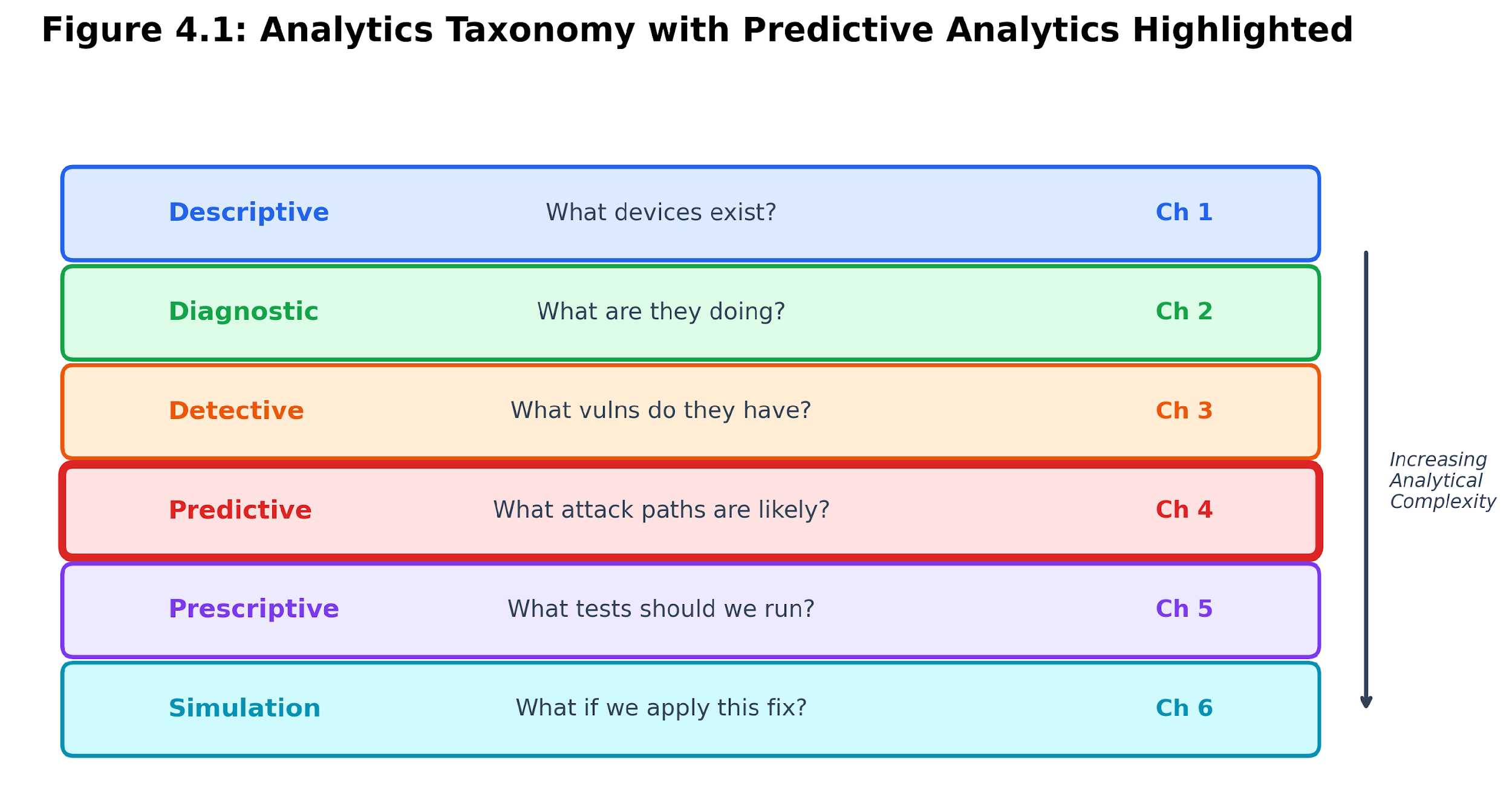
Figure 4.1: Analytics taxonomy. Attack graph analytics moves the course sequence from descriptive, diagnostic, and detective evidence toward predictive risk reasoning.
The key insight at the predictive level is that vulnerability severity, in isolation, is a poor predictor of organizational risk. CVSS assigns the same base score to every instance of CVE-2021-44228, regardless of the affected host's network location. An attack graph encodes what CVSS cannot: topology, reachability, potential for lateral movement, and physical consequences. Two devices with identical CVSS profiles can have wildly different BRS values because one is reachable in 2 hops from an internet-facing entry point. At the same time, the other is isolated behind 3 segmentation boundaries.
This chapter relies on five analytical tools:
-
Graph construction from scan results, encoding network topology and security relationships as a directed graph
-
Path analysis using Yen’s k-shortest paths to enumerate attack sequences that an adversary would follow.
-
Composite risk scoring that weights vulnerability, exploitability, reachability, physical consequence, supply chain, and compensating controls into a single metric
-
What-if simulation that clones the graph, applies hypothetical remediation actions, and measures the resulting risk delta.
-
External intelligence correlation that enriches internal findings with threat feeds and behavioral deviation detection
Instead of just listing vulnerabilities, this approach gives a ranked list of attack paths, detailed risk scores for each device (with a breakdown of risk factors), and a tool to preview how fixes might change the risk before making any changes.
4.2 Attack Graph Fundamentals
4.2.1 What Is an Attack Graph?
An attack graph is a special kind of network map. In it, nodes are network parts, and edges show possible routes an attacker could use. Unlike a regular network diagram, an attack graph highlights security details, like which devices run risky services, have known exploits, reuse credentials, or control physical processes.
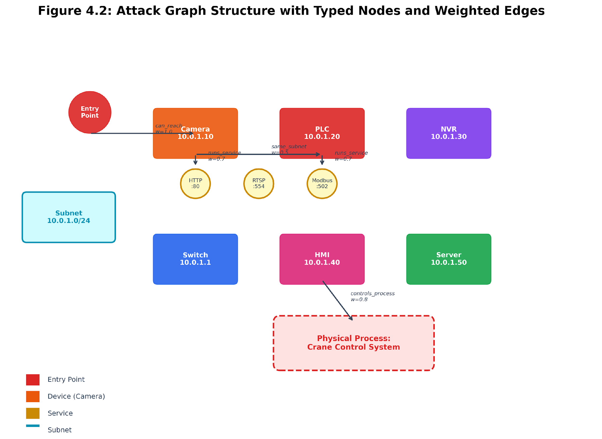
Figure 4.2: Attack graph overview. Devices, services, subnets, entry points, and physical processes form a directed graph whose edges encode the semantics of attacker movement.
The Breakwater attack graph uses five node types:
| device | device:192.168.86.42 | A discovered host | Google Nest Hub |
|---|---|---|---|
| service | service:192.168.86.42:8443 | An open service on a host | HTTPS on port 8443 |
| subnet | subnet:192.168.86.0/24 | A /24 network segment | Home network |
| entry_point | entry_point:192.168.86.1 | An internet-facing device | Gateway router |
| physical_process | physical_process: HVAC Control | A physical process controlled by a device | Building HVAC |
Table 4.2. Node types in the Breakwater attack graph.
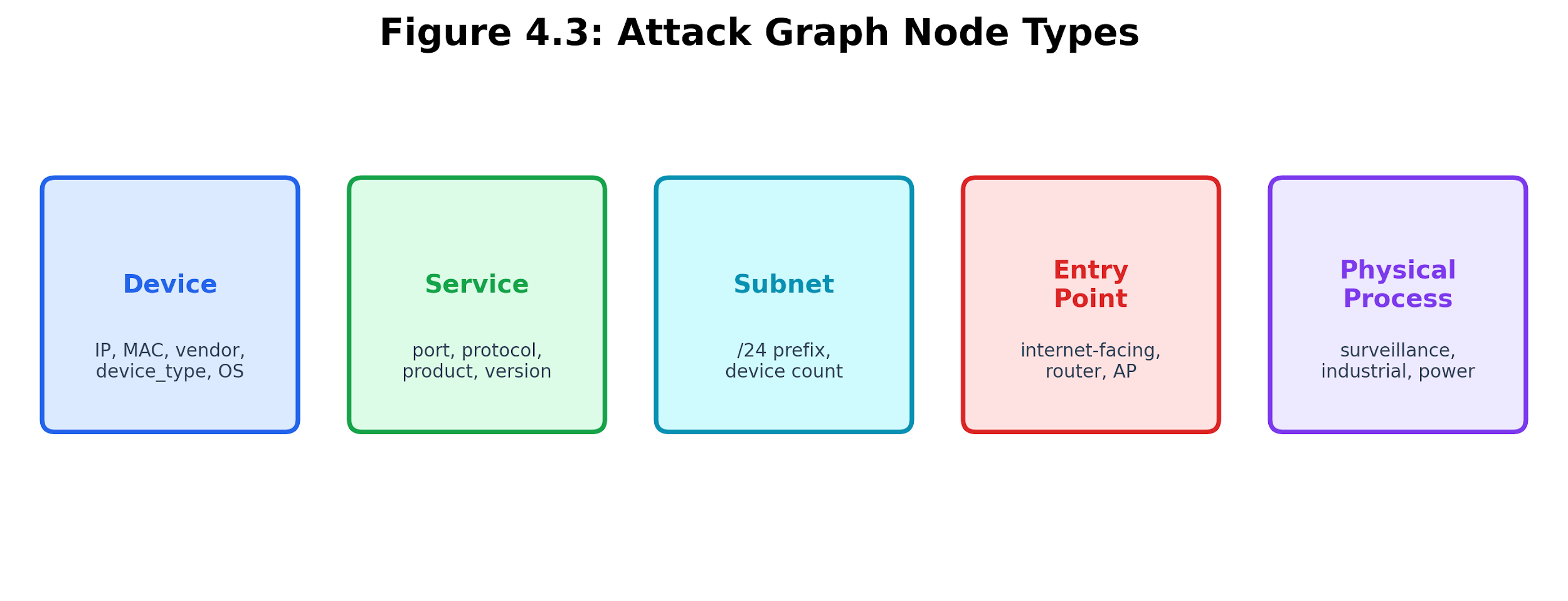
Figure 4.3: Node types in the Breakwater attack graph. The five node classes separate observed assets from services, network segments, entry points, and physical processes.
Each node holds information collected earlier. Device nodes include IP address, MAC address, vendor, device type, and operating system. Service nodes track port number, protocol, product, and version. Physical process nodes have a safety-critical flag that changes their risk score.
4.2.2 Edge Types and Weights
Edges in the attack graph show the connections an attacker could use to move through the network. Each edge type has a weight that measures how hard it is for an attacker to cross. Lower weights mean it is easier and faster for an attacker.
| shares_credentials | 0.1 | Two devices share default credentials – trivial lateral movement |
|---|---|---|
| exploitable_via | 0.3 | A service has a known CVE (adjusted by severity: critical=0.1, high=0.2, medium=0.4) |
| same_firmware | 0.4 | Two devices run identical firmware – one exploits chains to both |
| same_subnet | 0.5 | Devices on the same /24 – L2 adjacency enable ARP-based attacks |
| runs_service | 0.7 | Device exposes a network service – attack surface |
| communicates_with | 0.7 | Observed communication between devices |
| controls_process | 0.8 | Device controls a physical process – high-value target |
| can_reach | 1.0 | L3 routed reachability from the entry point – requires more effort |
Table 4.3. Edge types and their attacker-perspective weights.
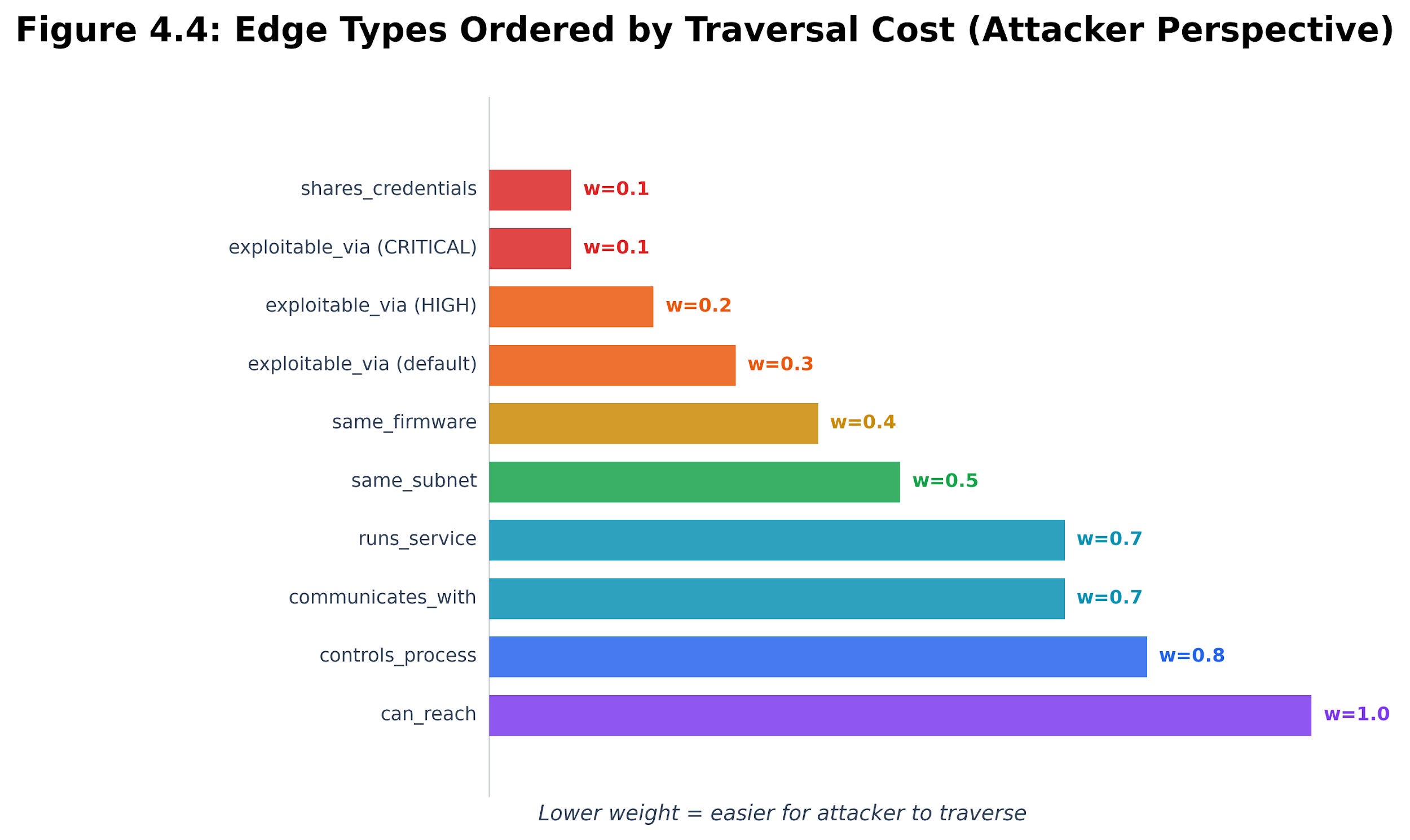
Figure 4.4: Edge weight comparison. Lower-weight relationships, such as shared credentials and critical exploits, are easier for an attacker to traverse than routed reachability or physical-process control.
These weights are set based on the effort required by an attacker. For example, credential reuse gets a low weight (0.1) because it is easy for an attacker to move between devices with the same credentials. A critical CVE with a public exploit also gets a weight of 0.1. Being on the same subnet is a bit harder (weight 0.5) because it may require ARP spoofing. Crossing into a different subnet is even harder (weight 1.0) because it usually means getting past firewalls or routing barriers.
These weights have sensible default values, but operators can change them using the BREAKWATER_BRS_WEIGHTS setting. For example, if the network perimeter is strong but internal segmentation is weak, the same subnet weight can be lowered to show that attackers can move more easily within the network.
4.2.3 Graph Construction Pipeline
The AttackGraphBuilder constructs the graph from scan results in eight sequential steps:
-
Add device nodes – One node per discovered host, carrying IP, MAC, vendor, device type, and OS metadata.
-
Add service nodes – One node per open service on each host, connected to its parent device via a runs_service edge.
-
Add subnet edges – Group devices by /24, create subnet nodes, and add bidirectional same_subnet edges between each device and its subnet.
-
Add credential-sharing edges – Find devices that share identical default credentials and add bidirectional shares_credentials edges between them.
-
Add firmware-sharing edges – Find devices running the same firmware version and add same_firmware edges.
-
Add exploit edges – For each CVE on a host, add an exploitable_via edge from the affected service to the parent device, with weight adjusted by severity.
-
Add physical-process edges: map device types to physical processes using a static lookup table, and add controls_process edges.
-
Mark entry points – Identify routers, gateways, access points, and devices with web services (ports 80, 443, 8080, 8443) as potential network entry points.
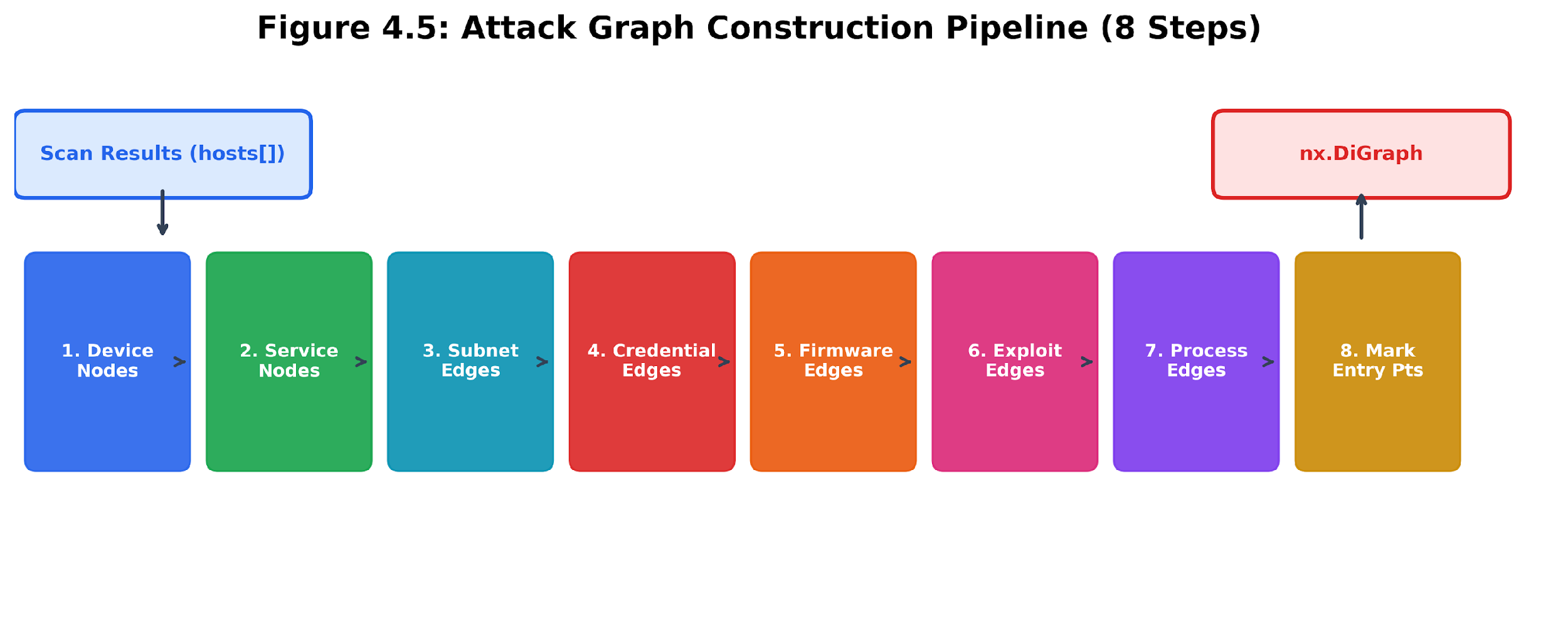
Figure 4.5: Attack graph construction pipeline. The builder turns scan results into a graph with devices, services, subnets, exploits, physical processes, and entry points in eight clear steps. The process is always the same: using the same scan results yields the same graph. This consistency helps analysts reach the same risk conclusions when using the same data.
In a typical home network with 21 devices, the attack graph has about 60-80 nodes and 100-150 edges. In a larger enterprise network with 500 hosts, the graph can have 2,000 to 3,000 nodes. NetworkX can build graphs of this size quickly—a 500-host graph typically takes less than 200 milliseconds.
Scaling up to networks with more than 500 hosts brings extra challenges. In networks with thousands of devices (like 3,000 hosts and over 10,000 nodes), memory use and path-finding can slow things down. On regular hardware, building the graph and analyzing attack paths may take a few seconds. NetworkX works well for mid-sized networks, but larger networks may require distributed graph tools or faster libraries such as igraph or graph-tool. To use resources better, you can limit the number of attack paths per target, split the graph for parallel analysis, or focus on high-value devices. For real-time or very large networks, incrementally updating the graph and calculating path metrics only when needed helps maintain high performance.
from apps.api.app.scanning.attack_graph.graph_builder import AttackGraphBuilder
builder = AttackGraphBuilder()
graph = builder.build(scan_id="abc123", hosts=scan_results)
# graph is a networkx.DiGraph
print(f"Nodes: {graph.number_of_nodes()}, Edges: {graph.number_of_edges()}")
4.3 Attack Path Analysis with Yen’s K-Shortest Paths
4.3.1 Why K-Shortest Paths?
A key question in attack graph analysis is: given the network layout and known vulnerabilities, what step-by-step routes could an attacker use to reach a valuable target from their entry point?
Finding only the shortest attack path is not enough. If that path is blocked, for example, by a quick patch, an attacker will look for the next best way in. To plan defenses effectively, you need to consider all realistic paths an attacker might take.
Yen’s algorithm is designed for this challenge. While Dijkstra’s algorithm finds only the single shortest path, Yen’s algorithm efficiently finds the top K shortest, loop-free paths between two points. Each path is ranked, giving you a list of the best alternatives, each at least as long as the previous one.
The algorithm works by iteratively finding deviations from previously discovered paths:
-
Find the shortest path P_1 using Dijkstra’s algorithm.
-
For each subsequent path P_k (k = 2, 3, …, K):
-
For each node in P_{k-1}, compute the shortest path from that node to the destination while avoiding edges used by previously found paths at the same prefix point.
-
Among all these “spur paths,” select the one producing the lowest-cost complete path.
-
Add this path to the result set.
In the Breakwater implementation, AttackPathEngine._k_shortest_paths wraps NetworkX’s shortest_simple_paths function, which implements a variant of Yen’s algorithm. The method computes up to K paths per source-target pair, with a configurable maximum hop count (default: 10) to prevent degenerate long paths.
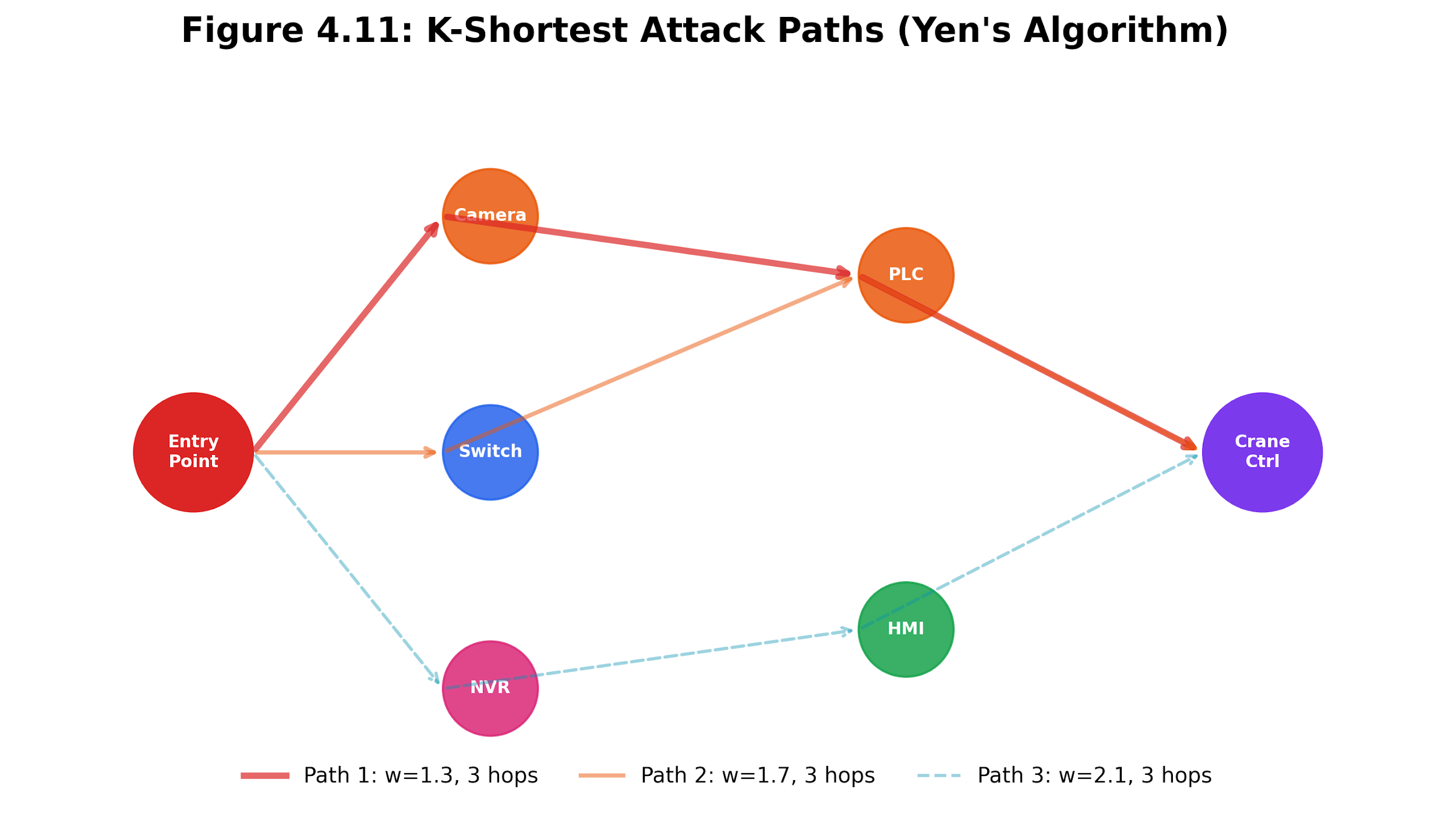
Figure 4.6: Yen’s k-shortest paths algorithm. The algorithm begins with the shortest path, then searches for spur-path deviations to enumerate alternate loopless attack routes.
4.3.2 Entry Points and High-Value Targets
Attack path analysis requires two inputs: where an attacker can enter, and what they want to reach.
Entry points are identified heuristically from device metadata:
-
Routers, gateways, access points, firewalls, and VPN devices (by device type)
-
Any device exposing web services on ports 80, 443, 8080, or 8443
These heuristics reflect the reality that internet-facing services are the most common initial access vector. The Breakwater engine adds an entry_point node for each qualifying device and connects it to the device node via a can_reach edge.
High-value targets are devices whose compromise would have a disproportionate impact:
-
Industrial control devices: PLCs, SCADA systems, HMIs, RTUs
-
Surveillance infrastructure: NVRs, DVRs
-
Physical security: access control systems, fire alarm panels
-
Data stores: NAS devices, servers
-
Hub devices: any device with 5 or more incoming graph edges (high in-degree indicates centrality)
The path engine then calculates the K shortest routes for each entry point-target pair. By default, it finds up to 5 paths per pair and caps the total at 50 per scan, always sorting them so the easiest paths rise to the top.
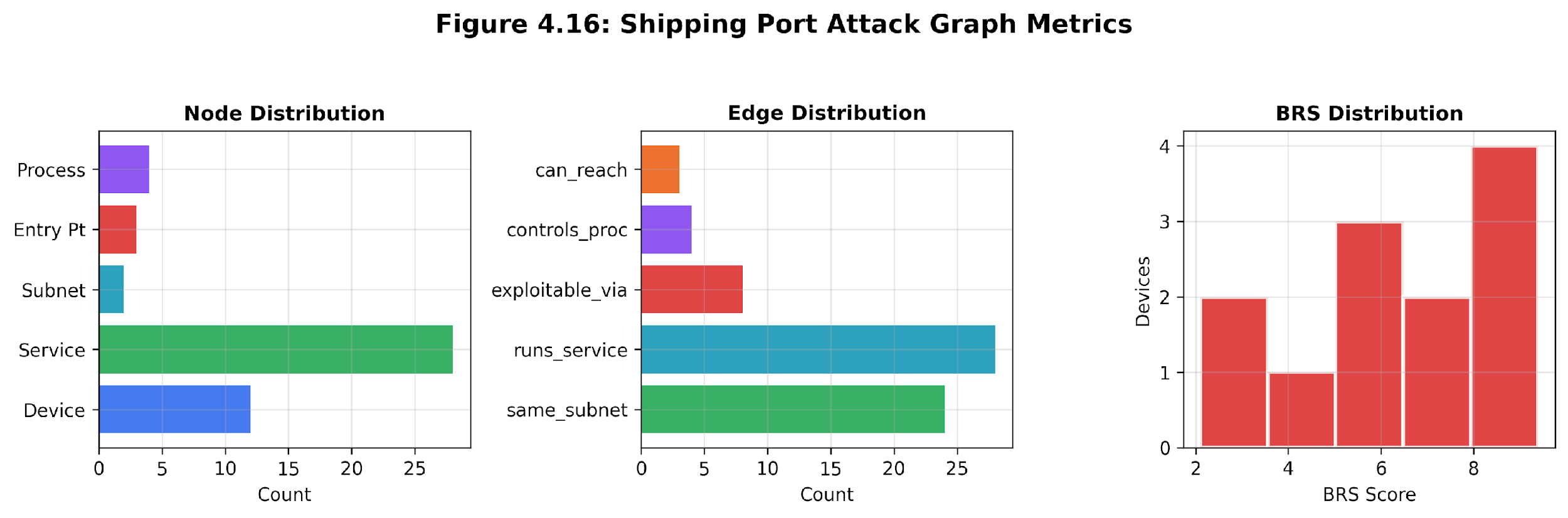
Figure 4.7: Attack graph metrics. Degree, centrality, path count, and reachability metrics summarize which devices shape the movement of attackers across the graph.
4.3.3 Path Probability and Time Estimation
Each attack path carries two derived metrics beyond total weight:
Probability. The probability that an attacker successfully traverses the complete path is modeled as:
P(path) = 1 / (1 + weight). For instance, a path with a total weight of 0.3, such as from the entry point to the same subnet to shared credentials, gets a probability of 0.77. A heavier path with weight 3.0 drops to 0.25. This reciprocal model was chosen for its simplicity and for producing a monotonic mapping where lower-weight paths are ranked higher, which is practical for prioritization. While this approach is not grounded in empirical attack data and does not estimate the true likelihood of compromise, it avoids overfitting and remains stable across varying path structures. More sophisticated models, such as logistic or Bayesian probability functions, could be explored to incorporate attacker profiles, exploit success rates, or defensive detection for research or advanced operational contexts. For now, this model provides a transparent, computationally light means of ranking paths, but its results should be interpreted as ordinal planning evidence rather than precise field probabilities.
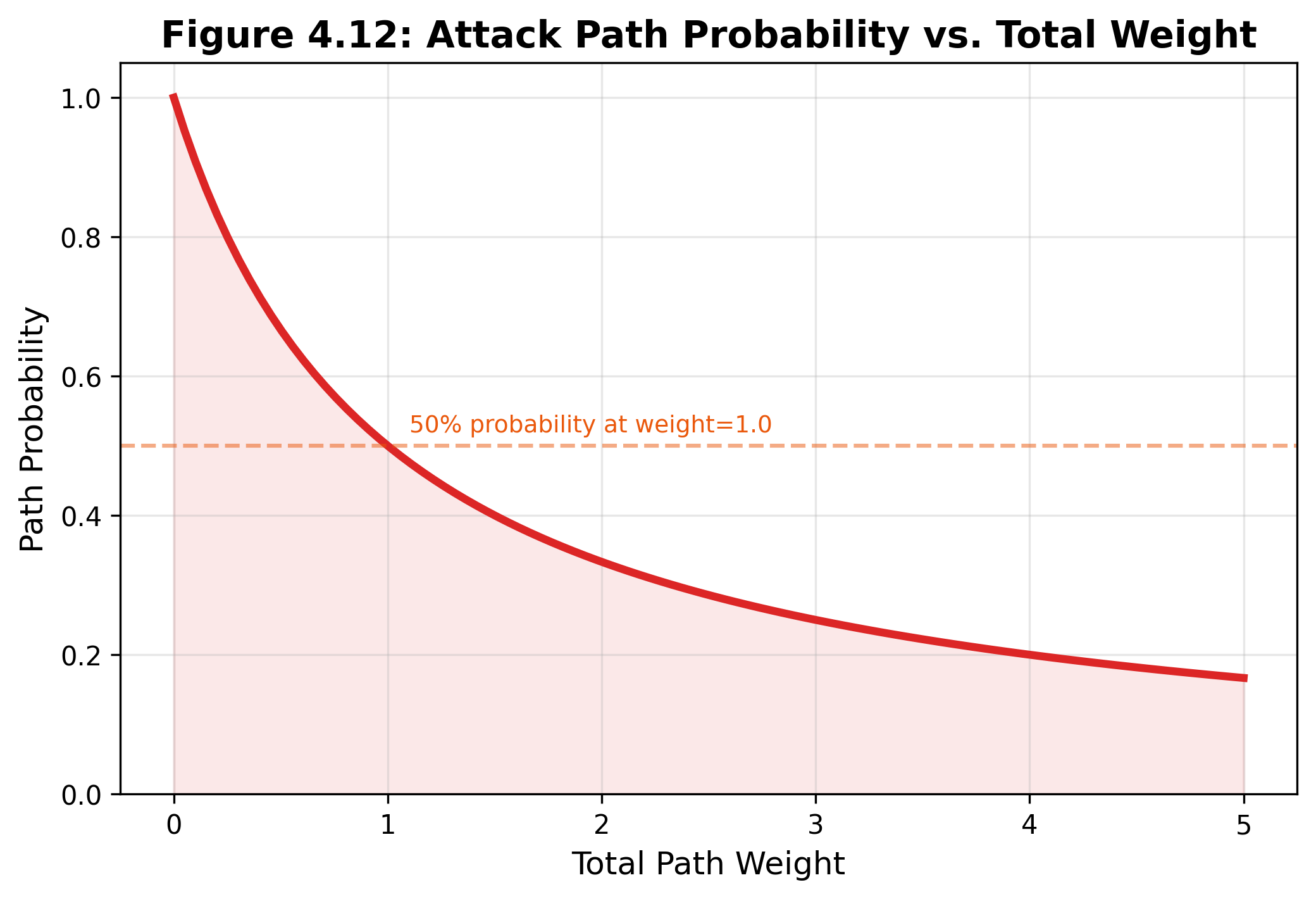
Figure 4.8: Attack path probability curve. The simple reciprocal model ranks low-weight paths as more probable while preserving an explicit limitation: it is ordinal planning evidence, not a calibrated field probability.
Estimated time. Each edge weight maps to an estimated traversal time in hours:
| 0.1 | 30 minutes | Default credentials: login attempt |
|---|---|---|
| 0.2 | 2 hours | Critical exploit: run Metasploit module |
| 0.3 | 4 hours | Known exploit: download and adapt PoC |
| 0.4 | 8 hours | Same firmware: reverse-engineer and reuse |
| 0.5 | 12 hours | Same subnet: ARP spoof, pivot |
| 0.7 | 24 hours | Service exposed: enumerate and probe |
| 0.8 | 48 hours | Physical process: understand industrial protocol |
| 1.0 | 72 hours | L3 routed: firewall bypass |
Table 4.4. Time-per-weight mapping for attack path estimation.
As edge weights go up, the estimated time to cross them also increases. For example, a three-hop path using shared credentials (0.1 + 0.1 + 0.5) might take about 12.5 hours, while a five-hop path through routed networks (1.0 + 0.7 + 0.5 + 0.3 + 0.8) could take up to 160 hours. These times are not exact, but they help you decide what to fix first: a 12-hour path needs faster action than one that would take a week to exploit.
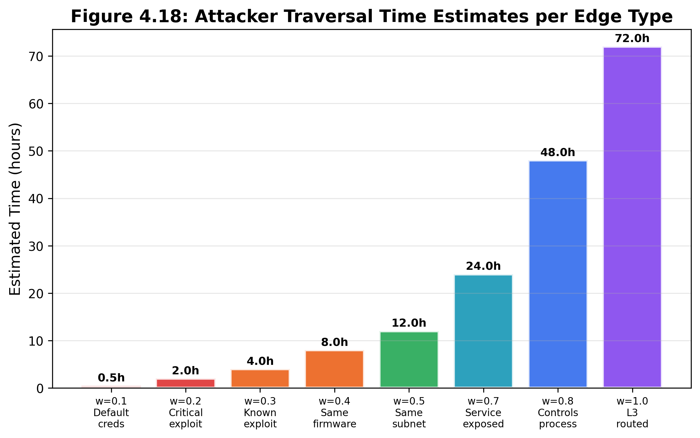
Figure 4.9: Time-per-weight relationship. Traversal time estimates increase as edge weight moves from default credentials and public exploits toward routed movement and physical-process understanding.
4.3.4 Critical Path Classification
A path is classified as critical when it satisfies two conditions:
-
Hop count <= 3 (short path)
-
Total weight < 2.0 (low difficulty)
Critical paths are the ones that need your immediate attention. For example, a two-hop route from an internet-facing router, through a shared credential, directly to a PLC (total weight: 0.1 + 0.1 = 0.2) is critical. On the other hand, a long seven-hop path through several firewalls (total weight: 5.6) is less urgent.
The AttackPathAnalysis result includes a critical_paths count that surfaces this classification to the dashboard. When the critical path count is nonzero, the scan report elevates the alert level.
4.4 Breakwater Risk Score (BRS)
4.4.1 The Composite Formula
Individual vulnerability scores (CVSS) assess a single CVE in isolation. The Breakwater Risk Score (BRS) assesses a device in its full operational context. BRS is a weighted composite of six factors:
BRS = w_V * V + w_E * E + w_R * R + w_P * P + w_S * S - w_C * C
Where:
-
V (Vulnerability surface, w=0.20): Derived from CVE count, maximum CVSS score, and volume factor. More severe CVEs produce a higher V.
-
E (Exploitability, w=0.20): Whether the vulnerabilities are actively exploited. Default credentials score 10.0 (maximum). CISA KEV entries score 9.0. High-severity CVEs without confirmed exploits score 6.0-8.0.
-
R (Reachability, w=0.20): Shortest weighted path from any entry point to this device. Closer to entry = more reachable = higher R. One hop from entry scores 10.0; ten hops score approximately 2.0.
-
P (Physical consequence, w=0.15): Whether the device controls a physical process. PLCs and SCADA systems score 10.0. Cameras score 6.0. Smart home devices score 4.0. IT-only devices score 0.0.
-
S (Supply chain, w=0.05): SBOM component risk from firmware analysis. Counts vulnerable components in the software bill of materials.
-
C (Compensating controls, w=0.20): Factors that reduce risk. Network segmentation adds 3.0. Current firmware adds 2.0. No default credentials adds 1.0. A few open ports add 1.0. This factor is subtracted from the score.
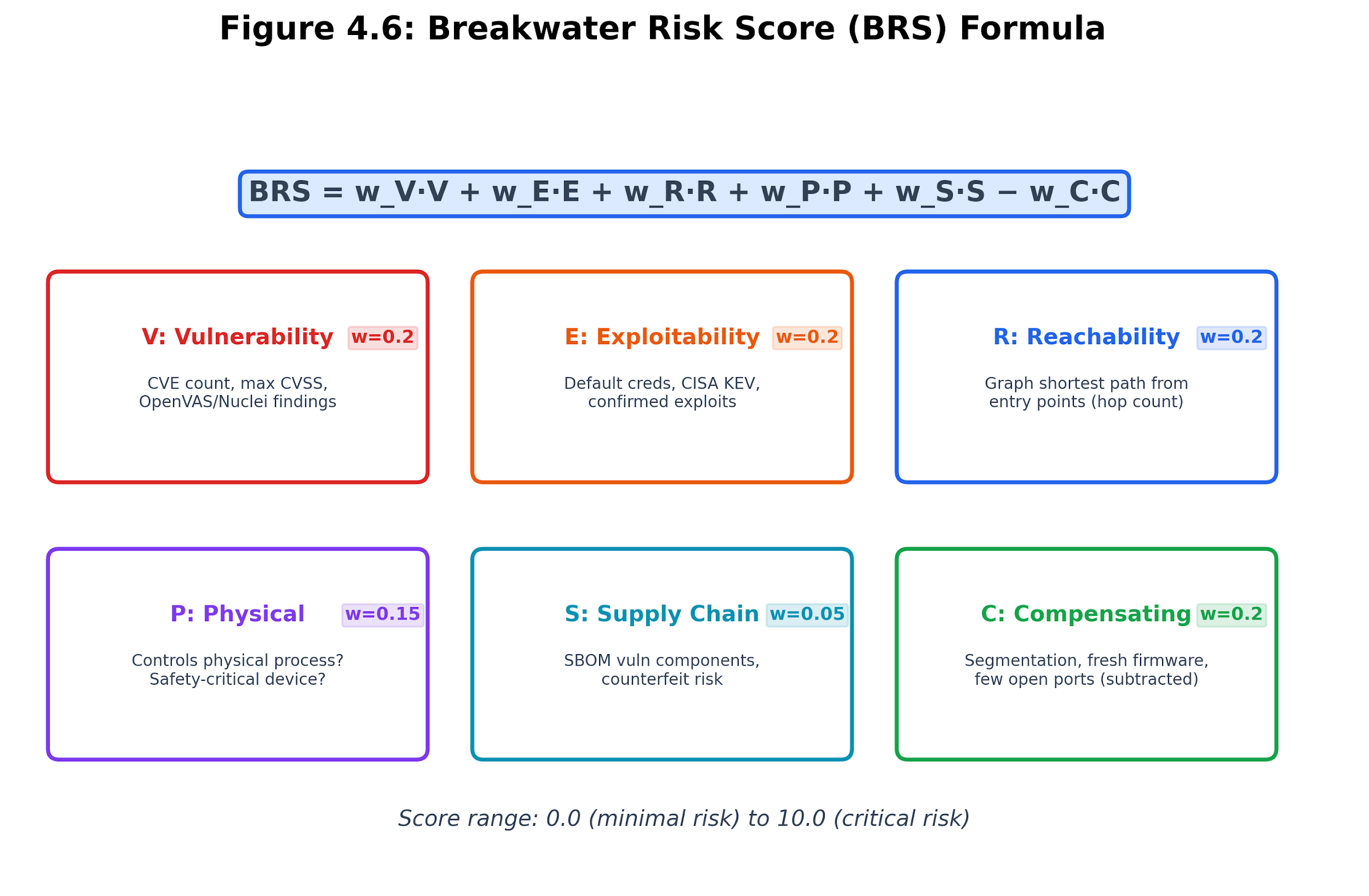
Figure 4.10: BRS formula decomposition. Vulnerability, exploitability, reachability, physical consequence, and supply-chain risk increase the score, while compensating controls reduce it.
The BRS is always kept between 0 and 10, and then turned into a clear rating:
| 9.0-10.0 | Critical | Immediate remediation required |
|---|---|---|
| 7.0-8.99 | High | Remediate within 7 days |
| 4.0-6.99 | Medium | Remediate within 30 days |
| 2.0-3.99 | Low | Monitor, schedule maintenance |
| 0.0-1.99 | Info | Acceptable risk |
Table 4.5. BRS rating thresholds and action levels.
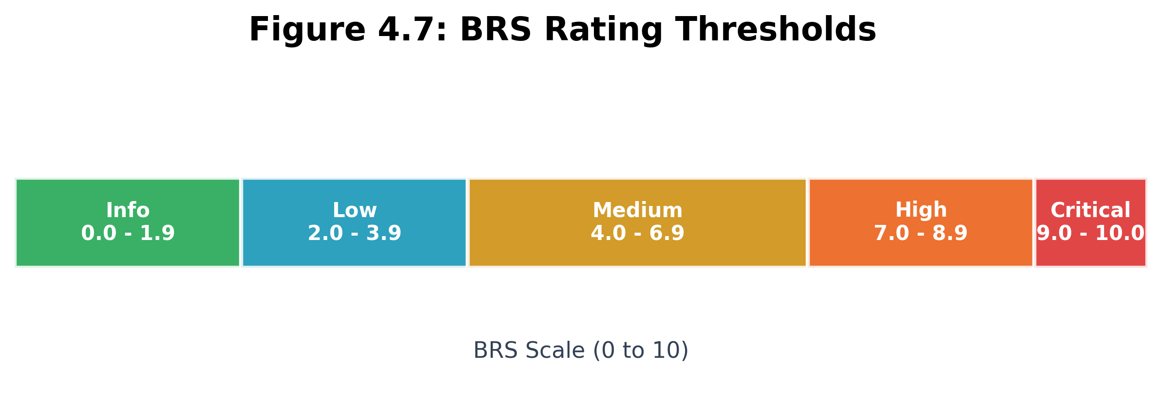
Figure 4.11: BRS rating thresholds. The 0-10 score maps to the Info, Low, Medium, High, and Critical operating bands, each with a different remediation urgency.
4.4.2 Why Reachability Matters More Than CVSS
Consider two devices on the same network:
-
Device A: IP camera with CVE-2021-36260 (Hikvision command injection, CVSS 9.8). Located on an isolated VLAN behind a firewall. No entry points on its subnet.
-
Device B: Smart thermostat with CVE-2023-XXXXX (CVSS 6.5, medium severity). One hop from the internet-facing router. Default credentials are active. Shares subnet with a PLC controlling HVAC.
CVSS alone ranks Device A as the higher priority (9.8 vs.6.5). BRS reverses this ranking:
-
Device A: V=9.8, E=8.0, R=0.0 (unreachable from entry points), P=6.0, S=0.0, C=3.0. BRS = 0.20×9.8 + 0.20×8.0 + 0.20×0.0 + 0.15×6.0 + 0.05×0.0 - 0.20×3.0 = 3.86 (low).
-
Device B: V=6.5, E=10.0 (default creds), R=10.0 (one hop), P=8.0 (HVAC controls), S=0.0, C=0.0 (no compensating controls). BRS = 0.20×6.5 + 0.20×10.0 + 0.20×10.0 + 0.15×8.0 + 0.05×0.0 - 0.20×0.0 = 6.50 (medium, bordering high).
The thermostat, despite its lower CVSS score, poses a greater risk because it is easily accessible, uses default credentials, and controls a physical process. The IP camera’s high CVSS score is less of a concern because network segmentation keeps it out of reach. This example shows why composite scoring that includes context gives a more accurate picture than CVSS alone.
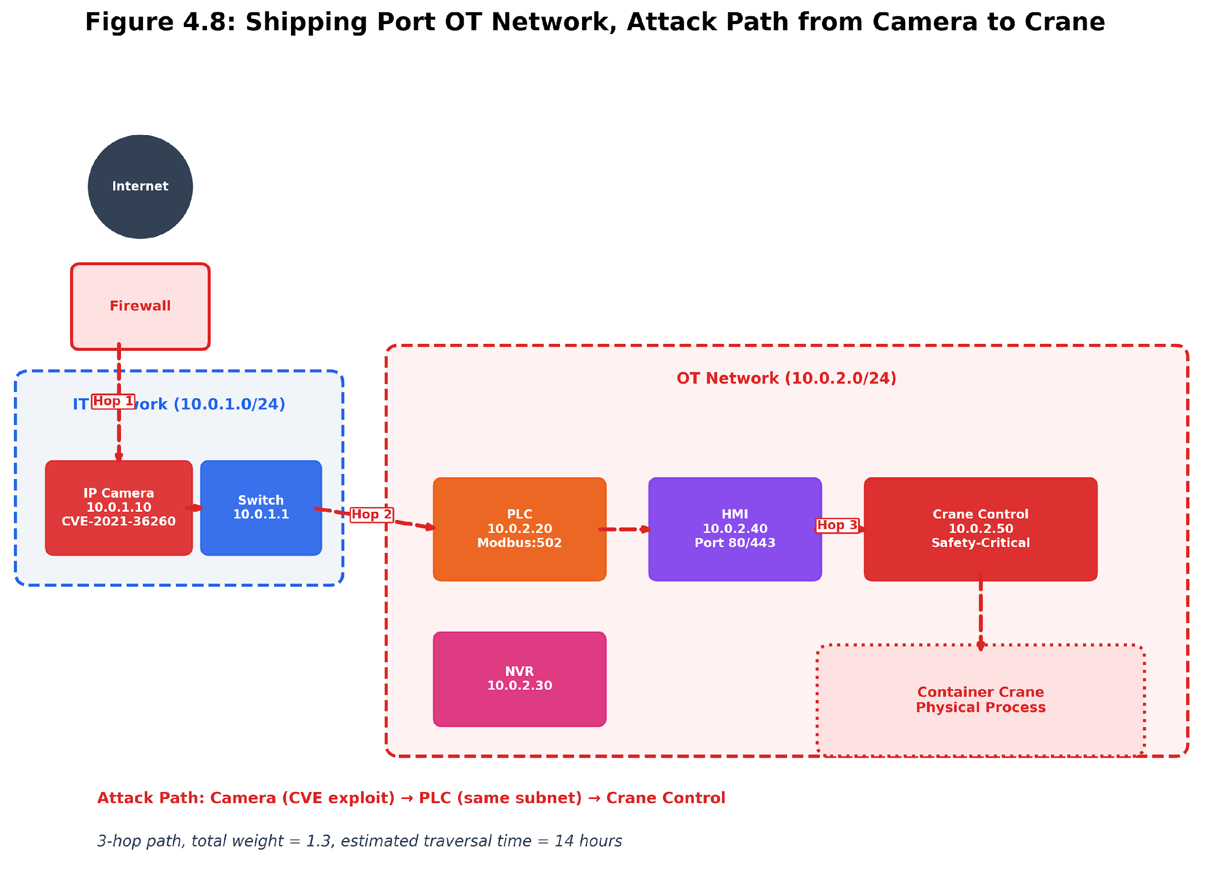
Figure 4.12: Shipping port scenario. The same vulnerability profile produces different operational risks when topology, physical consequences, and compensating controls are included.
4.4.3 BRS Factor Scoring Details
Vulnerability (V): The vulnerability score combines maximum CVSS severity with a volume factor:
V = min(10, max_cvss * volume_factor / 2 + max_cvss / 2)
volume_factor = min(1.0 + cve_count * 0.05, 2.0)
A device with a single critical CVE (CVSS 9.8) scores V = 9.8. A device with twenty critical CVE scores, V = 10.0 (capped). A device with only medium CVEs (CVSS 5.0, count 3) scores V = 5.0 * 1.15 / 2 + 5.0 / 2 = 5.375.
Exploitability (E): Scored by the most severe exploitability indicator:
-
Default credentials present: E = 10.0 (immediate, requires no exploit development)
-
CISA Known Exploited Vulnerability (KEV): E = 9.0 (confirmed active exploitation)
-
Critical CVE without confirmed exploit: E = 8.0
-
High CVE: E = 6.0
-
No exploitability indicators: E = 0.0
Reachability (R): Uses the shortest weighted path from any entry point to the device in the attack graph:
R = max(2.0, 10.0 - shortest_path_length * 0.8)
If no path exists (device is unreachable from all entry points), R = 0.0. One-hop distance (weight ~1.0) yields R = 9.2. Five-hop distance (weight ~3.0) yields R = 7.6. Beyond 10 hops, R approaches 2.0.
Physical consequence (P): A static lookup based on device type. PLCs, RTUs, and SCADA devices score 10.0 because their compromise can cause physical harm. Fire alarms and elevators score 9.0. HVAC and access control score 8.0. Cameras and NVRs score 6.0. UPS and PDU devices score 7.0. Smart home devices score 4.0. Generic IT devices score 0.0.
Supply chain (S): Based on SBOM analysis from firmware extraction. Each vulnerable component in the software bill of materials adds 2.0, capped at 10.0.
Compensating controls (C): An aggregation of defensive measures. Network segmentation or VLAN assignment adds 3.0. Current firmware (freshness score > 0.7) adds 2.0. Absence of default credentials adds 1.0. Two or fewer open ports add 1.0. Maximum C is 10.0.
4.4.4 SHAP-Style Factor Attribution:
A composite score is only useful if stakeholders can understand why a device received its rating. The BRS explainer breaks the score into per-factor contributions using a SHAP-style (SHAPley additive explanations) approach.
For every device, the explainer creates a waterfall chart that shows exactly how each factor changes the score. Factors such as vulnerabilities, exploitability, reachability, and physical consequences raise the score, while compensating controls lower it. Each component’s impact is its weight multiplied by its score, and all the components add up to the final BRS.
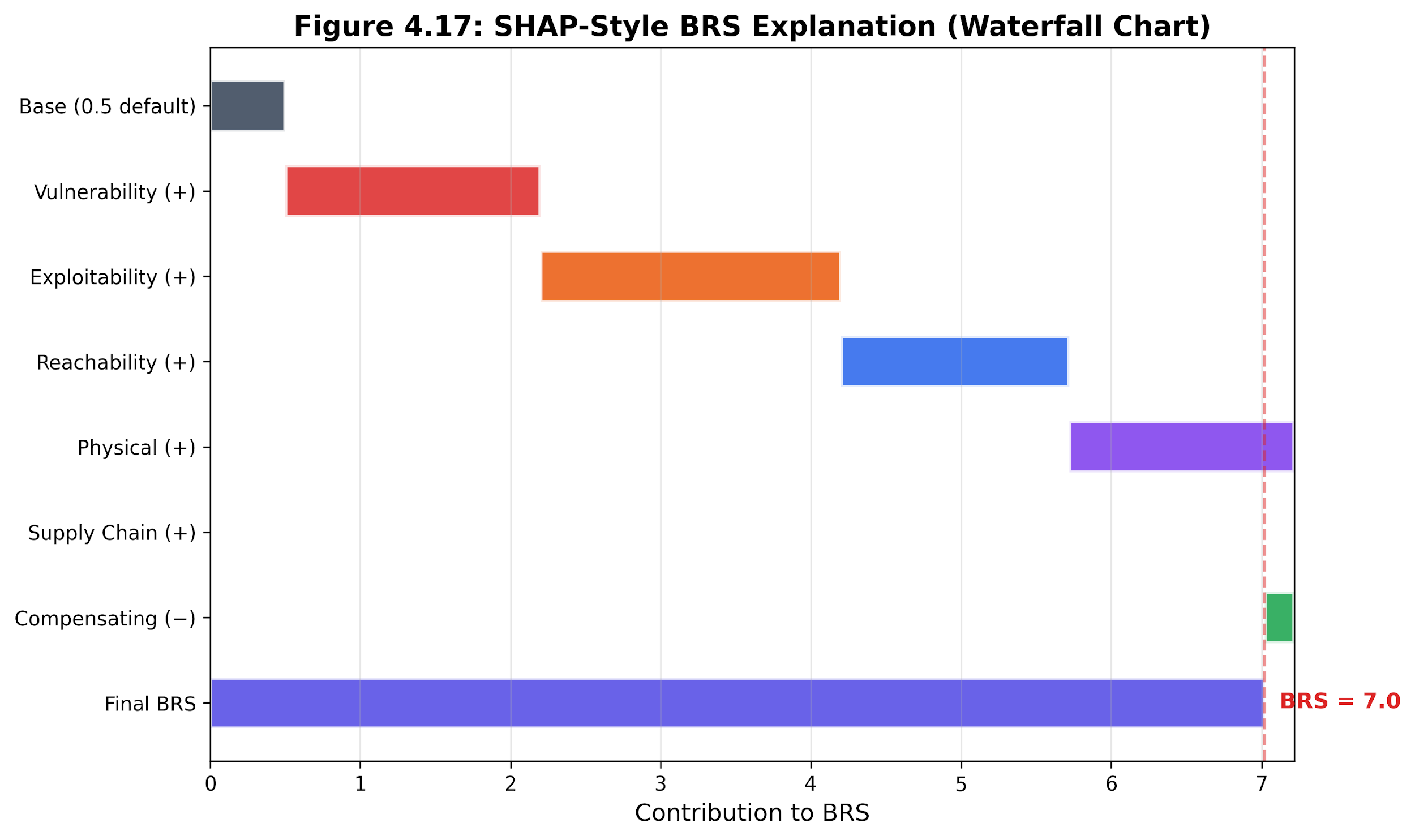
Figure 4.13: SHAP-style BRS waterfall. Positive factors raise device risk while compensating controls reduce the composite score, making the remediation lever visible.
This level of explainability matters in real operations. Suppose a device scores 7.8 on the BRS, with reachability adding 2.0 and compensating controls stuck at 0.0. The best fix is to add network segmentation, which boosts compensating controls and lowers reachability, rather than spending effort patching a medium-severity CVE that barely moves the needle.
For contrast, consider a second scenario where patching is the optimal action: an internet-facing web server is flagged with BRS 8.1. In this case, most of the score comes from a high vulnerability value (V=9.8) and exploitability (E=9.0) due to a critical CVE with a known exploit in the wild. At the same time, reachability is already high, and compensating controls are limited. Applying network segmentation here would require major infrastructure changes, whereas simply patching the vulnerable service dramatically reduces the vulnerability and exploitability factors, bringing the BRS below 5.0 and eliminating several attack paths.
These real-world scenarios illustrate how attributing the exact contributions of each BRS factor helps prioritize the right remediation action. Sometimes, architectural changes such as segmentation are the highest-impact fix; other times, rapid patching is the fastest way to drive down risk. By breaking down the score, BRS guides resource allocation with precision.
4.5 Behavioral Baselines
4.5.1 Why Baselines Matter
Chapters 1–3 give a snapshot from a single scan: what is on the network, what it looks like, and where the vulnerabilities are. But networks change over time. Devices come and go, ports open and close, and firmware gets updated or reset. A single scan cannot determine whether a port has always been open or appeared recently.
Behavioral baselines solve this by tracking device state across multiple scans. The BehavioralBaselineEngine maintains a per-device record of observed characteristics: open ports, service names, firmware version, device type, hostname, MAC address, and known CVEs. Each subsequent scan compares the current state against the baseline and flags deviations as anomalies.
This is temporal analysis in action. While the attack graph maps out spatial relationships—how things connect—the baseline engine tracks how things change over time. Together, they paint a much fuller picture of risk than either could alone.
4.5.2 Baseline Construction
The baseline is built incrementally. Each time a scan completes, the engine updates the baseline for every discovered device:
engine = BehavioralBaselineEngine()
# First scan: establishes baselines
result = engine.detect_network_anomalies(scan_1_hosts, scan_id="scan-001")
# result. Anomalies are empty (no previous data to compare)
# result.devices_baselined = 21
# result.new_devices = 21 (all new on first scan)
# Second scan: detects deviations
result = engine.detect_network_anomalies(scan_2_hosts, scan_id="scan-002")
# result.anomalies may contain: new_port, missing_device, firmware_change, etc.
Baselines are persisted to disk as JSON, keyed by IP address. Each DeviceBaseline record tracks:
| ip | string | Device identifier |
|---|---|---|
| observation_count | int | Number of scans where this device was observed |
| first_seen | ISO timestamp | The first scan that discovered this device |
| last_seen | ISO timestamp | Most recent scan |
| ports | list[int] | Open ports at the last observation |
| services | dict[port, name] | Service name per open port |
| hostname | string | Device hostname |
| device_type | string | Identified device type |
| firmware_version | string | Current firmware version |
| mac | string | MAC address |
| vendor | string | OUI vendor |
| has_default_creds | bool | Whether default credentials were found |
| cve_ids | list[string] | CVE IDs currently known |
Table 4.6. DeviceBaseline record structure.
The observation_count field serves as a confidence gate. The engine does not flag anomalies until a device has been observed at least twice (configurable via BREAKWATER_BEHAVIORAL_MIN_OBSERVATIONS). A device seen in only one scan has no baseline to deviate from.
4.5.3 Anomaly Detection
The baseline engine detects ten categories of anomaly:
| new_port | Medium | A port is open that was not open in previous scans |
|---|---|---|
| missing_port | Low | A previously open port is now closed |
| new_service | Medium | The service on a port changed (e.g., HTTP became SSH) |
| firmware_change | High | Firmware version changed between scans |
| type_change | High | Device type classification changed |
| hostname_change | Medium | Device hostname changed |
| new_cve | High | New CVEs were discovered on this device |
| credential_change | Critical | Default credentials appeared on a device that previously had none |
| new_device | Medium | A new device appeared on the network |
| missing_device | Medium | A previously observed device is no longer responding |
Table 4.7. Behavioral anomaly types and their default severity levels.
The severity assignments reflect operational significance. A credential change to “default credentials now present” is critical because it suggests the device was factory-reset, which could indicate either unauthorized physical access or a firmware update that reverted security settings. A new port is medium because it could indicate a legitimate configuration change or a compromise that opened a backdoor. A missing_port is low because closing a port generally reduces the attack surface.
Network-level anomalies go beyond individual devices. The engine also detects:
-
New devices: IPs observed in the current scan that have never been observed before. This catches unauthorized devices connected to the network.
-
Missing devices: IPs that were previously baselined (with sufficient observation count) but are absent from the current scan. This could indicate a device failure, removal, or a network segmentation change that makes the device unreachable.
4.5.4 Baseline-Enriched Risk Scoring
Behavioral anomalies feed back into the attack graph and BRS computation. A device with a credential_change anomaly (factory-reset detected) should have its exploitability score re-evaluated. A device with multiple new_port anomalies in rapid succession may indicate active compromise.
The integration works as follows:
-
Run the baseline engine on the current scan.
-
For each anomaly, annotate the affected host record with anomaly metadata.
-
Re-run BRS scoring with anomaly-adjusted factors.
-
The HYDRA engine (Section 4.10) incorporates behavioral signals into its temporal threat model.
This creates a feedback loop: scan data builds baselines, baselines detect anomalies, anomalies adjust risk scores, and adjusted scores inform remediation priorities.
4.6 Threat Intelligence Integration
4.6.1 The Intelligence Gap
Scan data tells you what is on your network and what vulnerabilities exist. It does not tell you whether anyone is actively targeting those vulnerabilities in the wild. A CVSS 7.5 vulnerability with no known exploit in the wild is a different priority than the same CVSS 7.5 vulnerability that CISA just added to its Known Exploited Vulnerabilities catalog because a ransomware group is using it.
Threat intelligence bridges this gap by bringing external context into internal risk assessment. The Breakwater ThreatIntelEngine consumes external feeds and correlates indicators with scan findings.
4.6.2 Feed Architecture
The threat intelligence system supports multiple feed types:
CISA KEV (Always-on). The Cybersecurity and Infrastructure Security Agency maintains a catalog of Known Exploited Vulnerabilities (CVEs) that have been confirmed to be actively exploited in the wild. Breakwater syncs this catalog via its public JSON endpoint. Each KEV entry includes the CVE ID, vendor, product, date added, remediation due date, and required action.
When a scan finds a CVE that appears in the KEV catalog, the ThreatIntelEngine produces a match with confidence 1.0 and severity “critical.” This match directly boosts the exploitability factor (E) in BRS to 9.0.
Custom STIX/TAXII feeds. Organizations with commercial or government threat intelligence subscriptions can configure additional feeds via the BREAKWATER_THREAT_INTEL_FEEDS environment variable. The feed configuration accepts:
[
{
"name": "Industry ISAC",
"url": "https://taxii.example.com/api/v2.1/collections/feeds/",
"feed_type": "stix",
"enabled": true
}
]
STIX (Structured Threat Information Expression) 2.1 is the standard format for exchanging cyber threat intelligence. TAXII (Trusted Automated Exchange of Intelligence Information) is the transport protocol. Together, they enable automated ingestion of indicators of compromise (IoCs): CVE IDs, malicious IP addresses, suspicious ports, domain names, and file hashes.
4.6.3 Indicator Types and Matching
The ThreatIntelEngine maintains five types of indicators:
| cve | Exact CVE ID match against scan findings | CVE-2021-44228 |
|---|---|---|
| ip | Exact IP match against discovered hosts | 203.0.113.42 |
| domain | Domain match against hostnames | evil.example.com |
| hash | File hash match against firmware analysis | SHA256 of the malicious binary |
| port | Open port match against service scan | Port 4444 (Meterpreter default) |
Table 4.8. Threat indicator types and matching strategies.
The matching engine runs after scan completion. For each host, it checks:
-
IP match: Is this host’s IP address in the indicator database? (Unusual for internal hosts, but relevant for internet-facing assets or known C2 infrastructure.)
-
CVE match: Do any of this host’s CVEs appear in the CISA KEV catalog or other threat feeds?
-
Port match: Does this host have open ports that match known malicious service indicators?
Each match produces a ThreatMatch with a confidence score (1.0 for exact CVE matches against KEV, lower for heuristic matches) and a description explaining the match.
4.6.4 Enriching BRS with Threat Intel
Threat intelligence matches adjust BRS in three ways:
-
Exploitability (E) boost: A CVE match against CISA KEV raises E to 9.0, regardless of the CVE’s base CVSS score. Active exploitation in the wild means the exploit is not theoretical.
-
Vulnerability (V) priority: Hosts with KEV-matched CVEs are flagged for immediate remediation in the scan report, superseding the normal rating-based prioritization.
-
Reputation scoring: The ReputationScorer computes a per-device reputation score based on the density and severity of threat intel matches. Devices with multiple KEV matches or that communicate with known-bad IPs receive lower reputation scores, which influence dashboard sorting and alert generation.
The HYDRA engine (Section 4.10) incorporates threat intelligence as a modifier on the exploitability stream, giving KEV-matched vulnerabilities an exponential moving average boost that persists across scan cycles.
4.7 What-If Simulation
4.7.1 The Remediation Planning Problem
Chapter 3 produced a vulnerability inventory. Section 4.4 scored those vulnerabilities in context. But which remediation actions should the organization execute first?
This is not a trivial question. Every remediation action has costs: direct cost (patching requires testing, credential rotation may break integrations), downtime (segmentation changes require maintenance windows), and opportunity cost (analyst time spent on one device is not spent on another). The optimal remediation plan maximizes risk reduction per unit of cost.
What-if simulation answers this by modeling the effect of remediation actions before they are executed. The WhatIfEngine takes a list of proposed actions, applies them to a cloned copy of the attack graph, re-scores all devices, and reports the risk delta.
Implementation Note: The WhatIfEngine evaluates proposed actions as a simulation. The computed deltas are approximations, not field-tested outcomes. Before accepting a recommendation, verify it against the actual device configuration and network policy.
4.7.2 Simulation Mechanics
The simulation follows a three-phase protocol:
-
Snapshot: Clone the current attack graph and host data.
-
Apply actions: Modify the cloned graph according to each remediation action.
-
Re-score: Compute BRS and attack paths on the modified graph.
-
Compare: Report the delta between original and simulated scores.
Five remediation action types are supported:
| patch | Remove all exploitable_via edges for the device | Clear CVE lists |
|---|---|---|
| segment | Remove same_subnet and can_reach edges | Mark the device as segmented |
| rotate_creds | Remove shares_credentials edges | Clear default credentials |
| disable_service | Remove the service node | Remove service from host record |
| firewall_rule | Remove all inbound edges (except from its own subnet node) | No change |
Table 4.9. Remediation action types and their effects on the simulation.
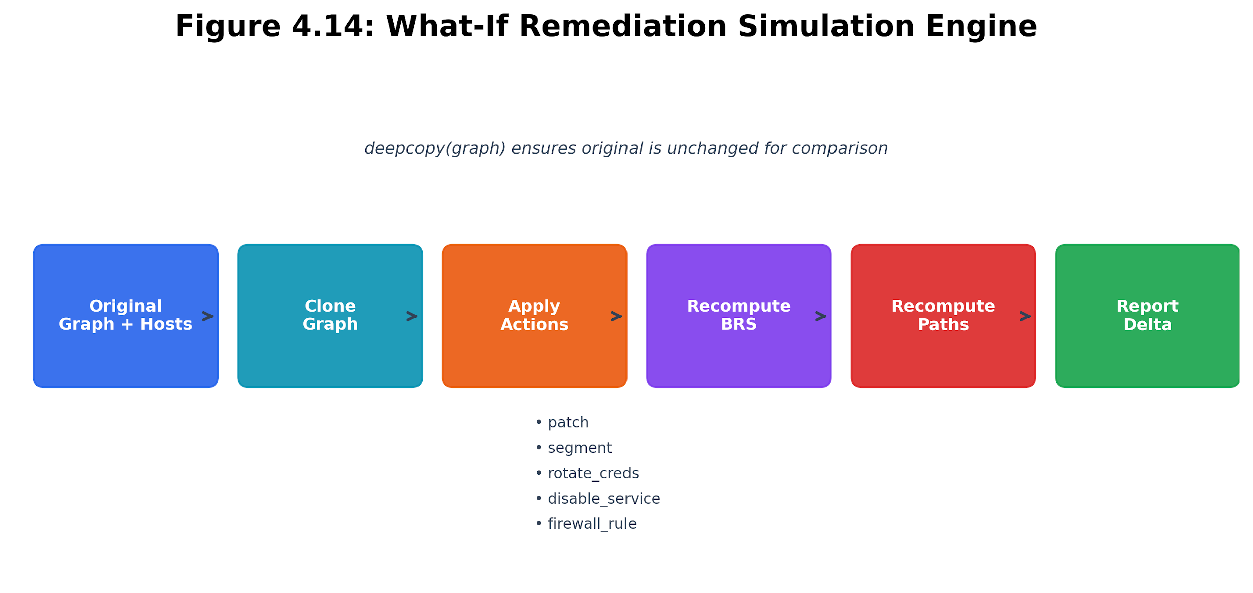
Figure 4.14: What-if simulation pipeline. The engine clones the graph state, applies candidate remediations, re-scores risk, and reports the predicted delta before production change.
Each action also includes a cost estimate (on a 1-10 scale) and an estimated downtime in hours. These values are configurable but have sensible defaults: credential rotation is cheap (cost 1.0, downtime 0.5 hours) while network segmentation is expensive (cost 5.0, downtime 4.0 hours). Cost and downtime estimates are derived from a combination of typical operational experience, vendor documentation, and in-lab measurement—credential changes are often quick administrative tasks. At the same time, segmentation may require equipment reconfiguration and scheduled maintenance. Students and analysts can tailor these estimates by factoring in their own environment-specific inputs, such as change management policies, average remediation times, or resource availability. All costs are intended as guidelines and can be adjusted via configuration to reflect local conditions or organization-specific priorities.
4.7.3 Example: Simulating Credential Rotation
Consider a network in which five IP cameras use the default credentials admin/admin. The attack graph has shares_credentials edges between all five cameras (10 bidirectional edges). From an entry point, an attacker can reach any camera through the credential-sharing cluster in two hops.
Simulation request:
{
"actions":[
{
"action_type":"rotate_creds",
"target_ip":"192.168.86.10",
"description": "Rotate credentials on camera 1"
},
{
"action_type":"rotate_creds",
"target_ip":"192.168.86.11",
"description": "Rotate credentials on camera 2"
}
]
}
Simulation result:
{
"original_score":6.42,
"simulated_score":4.18,
"delta":2.24,
"original_paths":23,
"simulated_paths":11,
"paths_eliminated":12
}
Rotating credentials on just two of five cameras removes 12 attack paths and reduces the average BRS by 2.24 points. The per_device_delta array shows which specific devices benefited most from the change.
4.7.4 Optimal Remediation Planning
The WhatIfEngine.generate_optimal_plan method automates remediation prioritization using a greedy algorithm:
-
Generate candidate actions for all hosts (patch if it has CVEs, rotate creds if defaults, segment if critical device type, turn off if insecure service).
-
For each candidate, simulate it in isolation and measure BRS reduction.
-
Select the candidate with the highest efficiency (BRS reduction/cost).
-
Apply it to the working graph.
-
Repeat until the budget is exhausted or no further improvement is possible.
This is a greedy approximation to the NP-hard budget-constrained optimization problem. It does not guarantee the global optimum, but in practice, it produces plans that are close to optimal. The key insight is that remediation actions have diminishing returns: the first credential rotation on a shared-credential cluster eliminates more paths than the fifth.
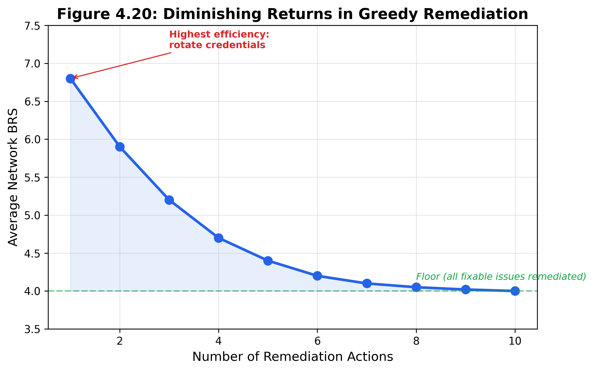
Figure 4.15: Remediation efficiency chart. Each remediation type is compared by BRS reduction per cost unit, showing that high-yield actions are not always the most expensive.
The output is a RemediationPlan with ranked actions, total cost, total downtime, projected average BRS after all actions, and overall efficiency score. This plan can be exported to a ticketing system (Jira, ServiceNow) for execution tracking.
4.8 MITRE ATT&CK ICS Mapping
4.8.1 From Vulnerabilities to Adversary Techniques
A CVE tells you what is broken. MITRE ATT&CK tells you how an adversary would use it. The ATT&CK framework for Industrial Control Systems (ICS) catalogs adversary techniques organized by tactic – the adversary’s objective at each stage of an intrusion.
The Breakwater MitreMapper translates scan findings into ATT&CK ICS technique mappings using three strategies:
CWE-based mapping. Each CVE is associated with one or more Common Weakness Enumerations (CWEs). The mapper maintains a static lookup from CWE to ATT&CK technique. For example, CWE-798 (Use of Hard-coded Credentials) maps to T0812 (Default Credentials) and T0891 (Hardcoded Credentials).
Device-type-based mapping. Device types imply potential technique applicability. A PLC implies susceptibility to T0821 (Modify Controller Tasking), T0836 (Modify Parameter), and T0835 (Manipulate I/O Image). A camera implies T0801 (Monitor Process State) and T0852 (Screen Capture).
Finding-type-based mapping. Specific scan findings map directly to techniques. A “default_credentials” finding maps to T0812 with confidence 1.0. An “insecure_protocol” finding (Telnet, FTP) maps to T0869 (Standard Application Layer Protocol).
Each mapping carries a confidence score reflecting the certainty of the association:
-
CWE-based: 0.7 (indirect but systematic)
-
Device-type based: 0.5 (inferred from device category)
-
Finding-type based: 0.8-1.0 (direct observation)
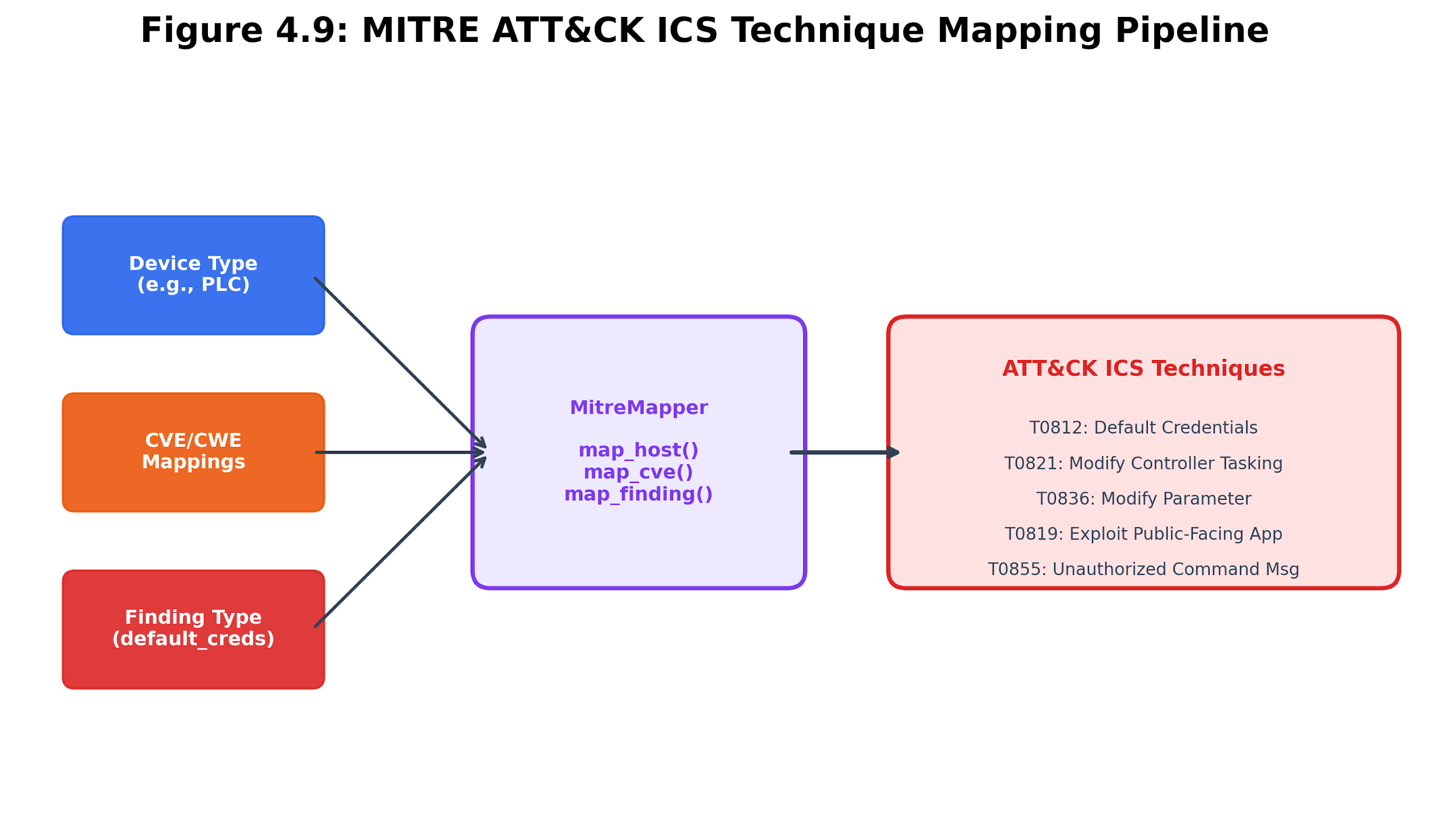
Figure 4.16: MITRE ATT&CK ICS mapping strategies. Finding-type, CWE-based, and device-type mappings carry different confidence levels because they rest on different evidence.
4.8.2 Scan-Level MITRE Coverage
The MitreMapper.map_scan method produces a scan-level summary:
-
Total mappings: How many technique instances were identified across all hosts
-
Unique techniques: How many distinct ATT&CK techniques were mapped
-
Technique counts: How many hosts does each technique apply to
-
Tactic counts: How many hosts does each tactic phase cover?
-
Per-host mappings: Which techniques apply to each specific device
This summary answers the question: “Which ATT&CK tactics does our network exposure cover?” If the scan reveals techniques spanning Initial Access, Lateral Movement, and Impact but nothing in Evasion or Persistence, that pattern suggests the attacker model is most likely to succeed against this network.
4.8.3 ICS-Specific Tactics
The ATT&CK ICS framework defines tactics specific to industrial environments:
| initial_access | Gain first foothold | T0819: Exploit Public-Facing Application |
|---|---|---|
| execution | Run adversary code | T0807: Command-Line Interface |
| persistence | Maintain access | T0839: Module Firmware |
| evasion | Avoid detection | T0820: Exploitation for Evasion |
| discovery | Learn about the environment | T0846: Remote System Discovery |
| lateral_movement | Move to other systems | T0812: Default Credentials |
| collection | Gather target data | T0802: Automated Collection |
| command_and_control | Maintain C2 channel | T0869: Standard Application Layer Protocol |
| inhibit_response_function | Prevent operator response | T0804: Block Reporting Message |
| impair_process_control | Disrupt the physical process | T0836: Modify Parameter |
| impact | Cause damage | T0879: Damage to Property |
Table 4.10. ATT&CK ICS tactics and their objectives.
4.9 STIX 2.1 Export
4.9.1 Why STIX?
Organizations do not operate in isolation. Threat data from one scan may be relevant to partners, regulators, or industry ISACs (Information Sharing and Analysis Centers). STIX (Structured Threat Information Expression) 2.1 provides a standardized format for sharing structured threat intelligence.
The Breakwater STIXExporter produces a STIX 2.1 bundle containing:
-
Identity object: Identifies Breakwater as the producing system
-
Attack-pattern objects: One per unique ATT&CK technique mapped in the scan
-
Vulnerability objects: One per CVE discovered on any host
-
Observed-data objects: One per host, referencing IPv4 address objects.
-
Relationship objects: Linking vulnerabilities to observed data (targets), observed data to addresses (observed)
-
Report object: A container referencing all other objects, representing the complete scan
Each attack-pattern object includes external references to the MITRE ATT&CK website and kill-chain-phase annotations linking the technique to its ICS tactic.
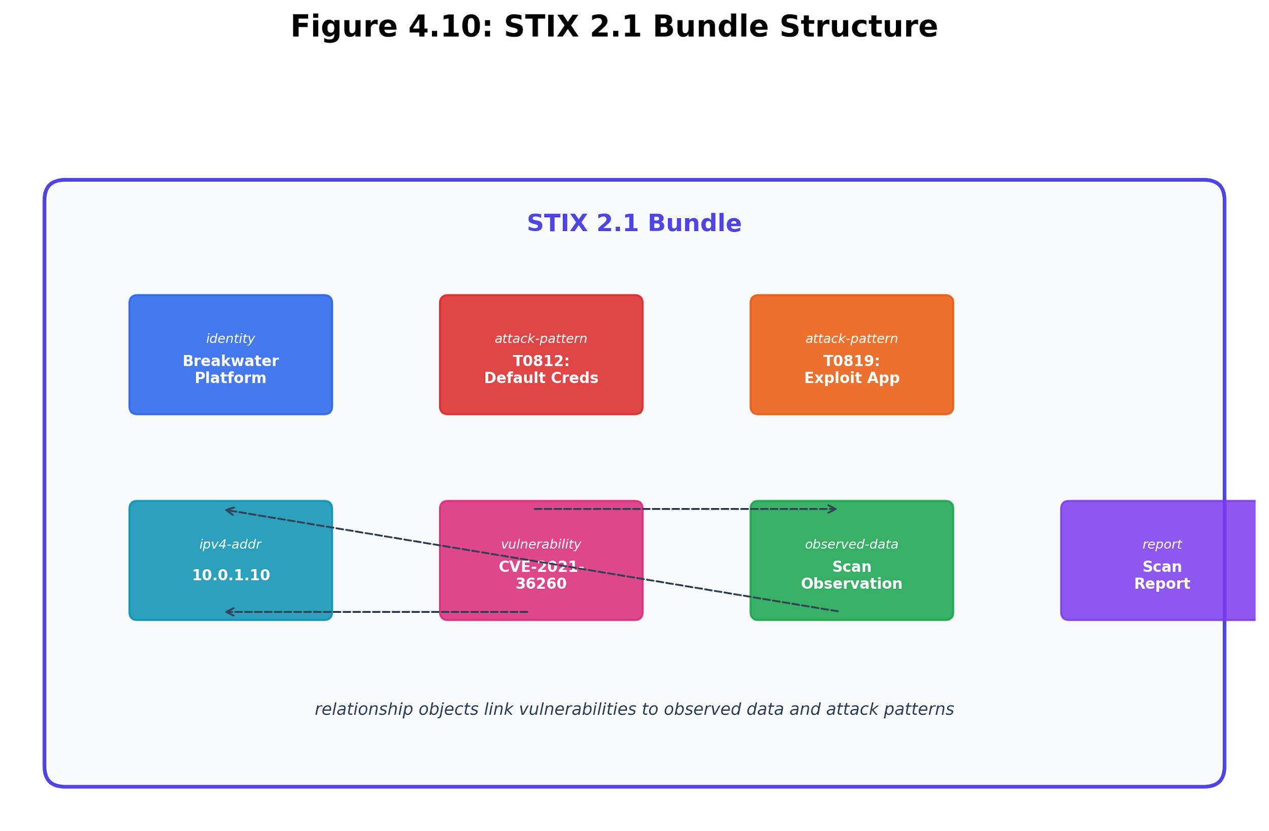
Figure 4.17: STIX 2.1 - bundle structure. Breakwater exports identities, collected data, vulnerabilities, attack patterns, relationships, and a report object as a shareable bundle.
4.9.2 Compliance and sharing.
STIX export serves three operational purposes:
-
Regulatory compliance: Frameworks like NIST CSF 2.0 and the EU CRA (Cyber Resilience Act) require structured vulnerability and threat documentation. STIX bundles provide auditable, machine-readable evidence.
-
Intelligence sharing: ISACs and government entities accept STIX/TAXII feeds. Exporting scan findings as STIX enables bidirectional intelligence sharing: the organization contributes indicators and receives context from sector partners.
-
Tool interoperability: STIX is consumed by SIEMs, threat intelligence platforms, and incident response tools. Exporting in STIX format allows Breakwater findings to flow into existing security operations workflows.
4.10 HYDRA Cross-Phase Analytics
4.10.1 Beyond Six Factors
The BRS formula in Section 4.4 uses six factors from Phases 1-7. The HYDRA engine extends this to eight factors by incorporating signals from all twelve intelligence streams in the Breakwater pipeline:
BRS_HYDRA = w1*V + w2*E + w3*R + w4*P + w5*S + w6*Q + w7*D - w8*C
The two additional factors:
-
Q (Quantum vulnerability, w=0.05): From Chapter 7, assessing the device’s exposure to quantum computing threats, such as RSA key lengths and post-quantum readiness.
-
D (Deception intelligence, w=0.05): From Chapter 10, measuring honeypot interaction signals near this device. High deception activity suggests active reconnaissance.
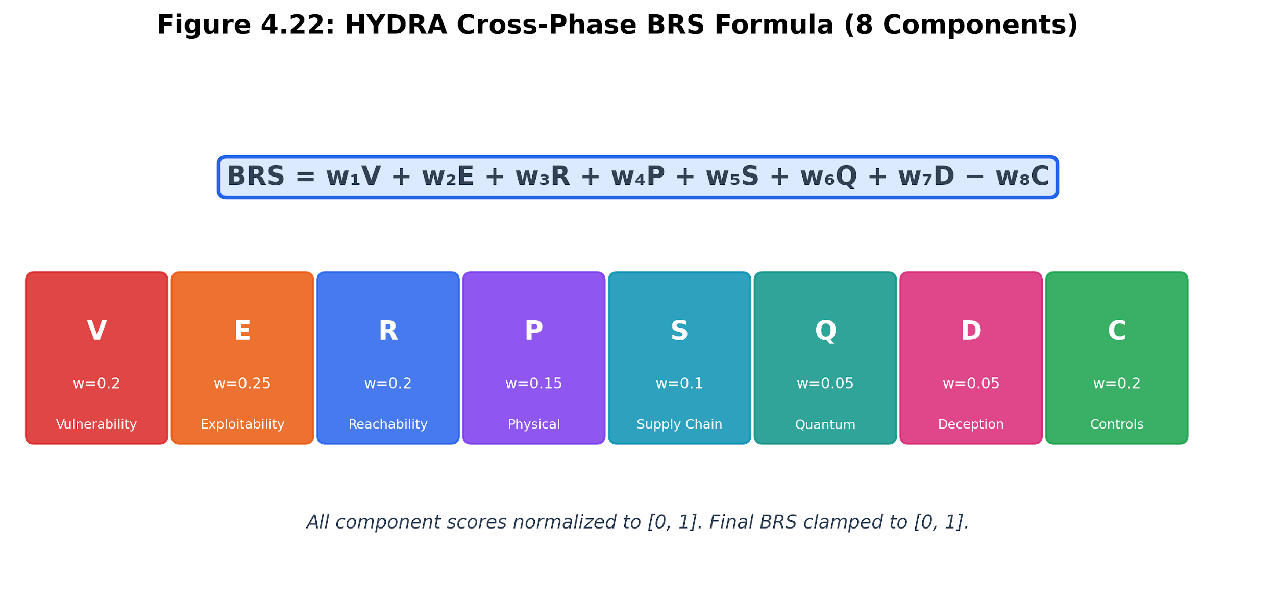
Figure 4.18: HYDRA BRS formula. The cross-phase score extends BRS by incorporating quantum-readiness and deception-intelligence streams while preserving compensating controls as a mitigating factor.
HYDRA normalizes all scores to [0, 1] and uses exponential moving averages to blend new stream data with historical observations (70% new, 30% historical). This means the BRS evolves as new scan data arrives, rather than resetting on each scan.
4.10.2 Temporal Threat Model
Each device maintains a DeviceThreatModel with a history of BRS observations. This enables two temporal analyses:
Risk regression detection: Has a device that was remediated (BRS dropped below 0.3) later become vulnerable again (BRS rose above 0.6)? This catches devices where patches were reverted, credentials were reset to defaults, or new vulnerabilities were discovered in updated firmware.
Predictive timeline: Given the historical BRS trajectory, what is the projected BRS in 30, 90, or 365 days assuming no remediation? The HYDRA engine models this using logistic growth: BRS increases slowly at first, then accelerates as unpatched vulnerabilities age and new exploit tools emerge, then saturates at 1.0.
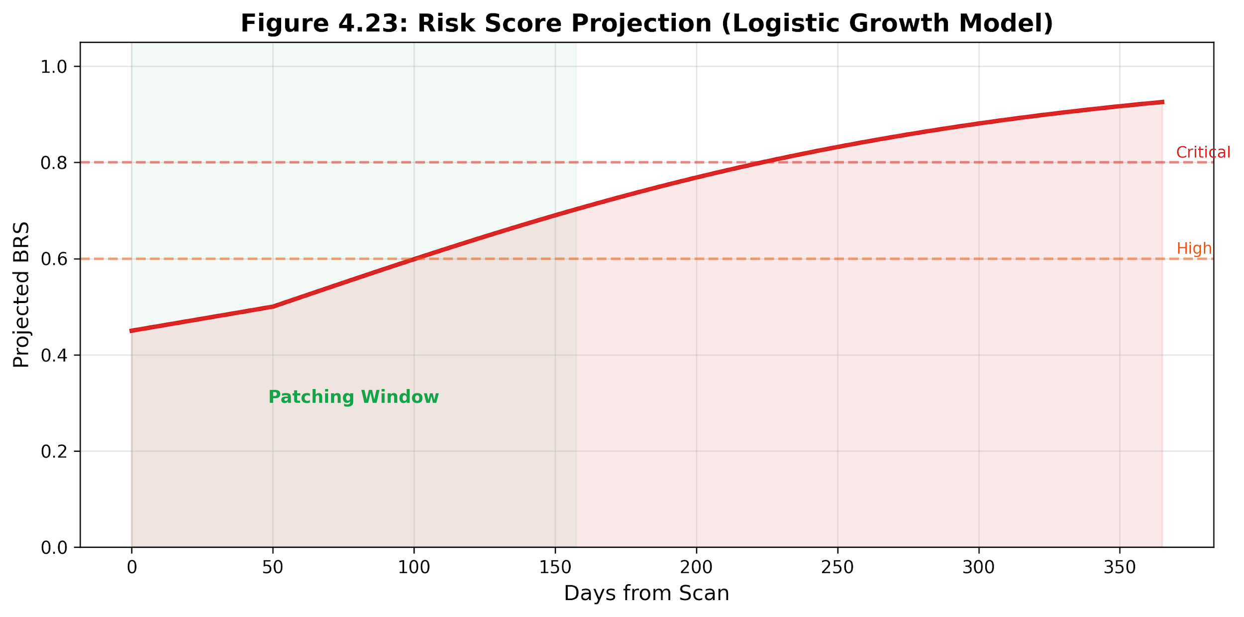
Figure 4.19: Risk timeline projection. Historical BRS observations support a bounded forecast that marks when a device is expected to cross the high-risk threshold.
4.10.3 GNN-Augmented Scoring
For organizations with PyTorch Geometric installed, the BRS engine can augment rule-based scoring with a Graph Neural Network:
Architecture. The GNNBRSModel uses two layers of heterogeneous graph attention convolution (GATConv via HeteroConv) followed by a readout MLP. The model learns from five edge types: same_subnet, has_service, exploitable_via, shares_credentials, and same_firmware.
Feature encoding. Each device is encoded as a 32-dimensional feature vector: port count (1), CVE count (1), max CVSS (1), default credentials flag (1), device type one-hot (8 categories), open port bitmap (16 top ports), and 4 padding dimensions.
Self-supervised training. The GNN is trained using rule-based BRS scores as pseudo-labels. A physics-informed loss function enforces monotonicity constraints: devices with more CVEs should have higher BRS. The final prediction blends GNN output (70%) with rule-based output (30%).
Value proposition. The GNN captures topological features that rule-based scoring cannot: devices that are structurally similar in the graph (similar neighborhoods, similar connectivity patterns) receive similar scores even if their individual attributes differ. This improves scoring for devices that lack some enrichment data.
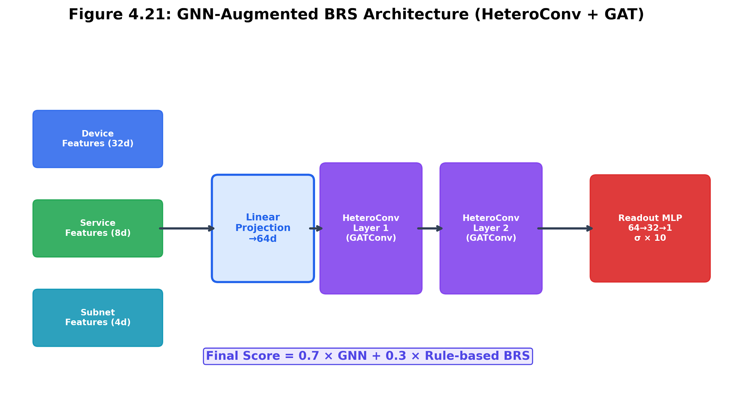
Figure 4.20: GNN-augmented BRS architecture. Device features and heterogeneous graph edges are fed into graph attention layers, which are then blended with rule-based scoring.
4.11 Network Segmentation Scoring
The AttackPathEngine.segmentation_score method quantifies the network segmentation quality on a 0-10 scale.
The computation examines graph connectivity:
-
Count the number of subnet nodes. A single-subnet network scores 0.0 (no segmentation).
-
Count device-to-device edges that cross subnet boundaries (source and destination are on different /24 networks).
-
Compute the cross-subnet ratio: cross_subnet_edges / total_device_edges.
-
Score: 10.0 * (1.0 - ratio).
A perfectly segmented network (no cross-subnet device-to-device edges) scores 10.0. A flat network where every device shares credentials with devices on other subnets scores close to 0.0.
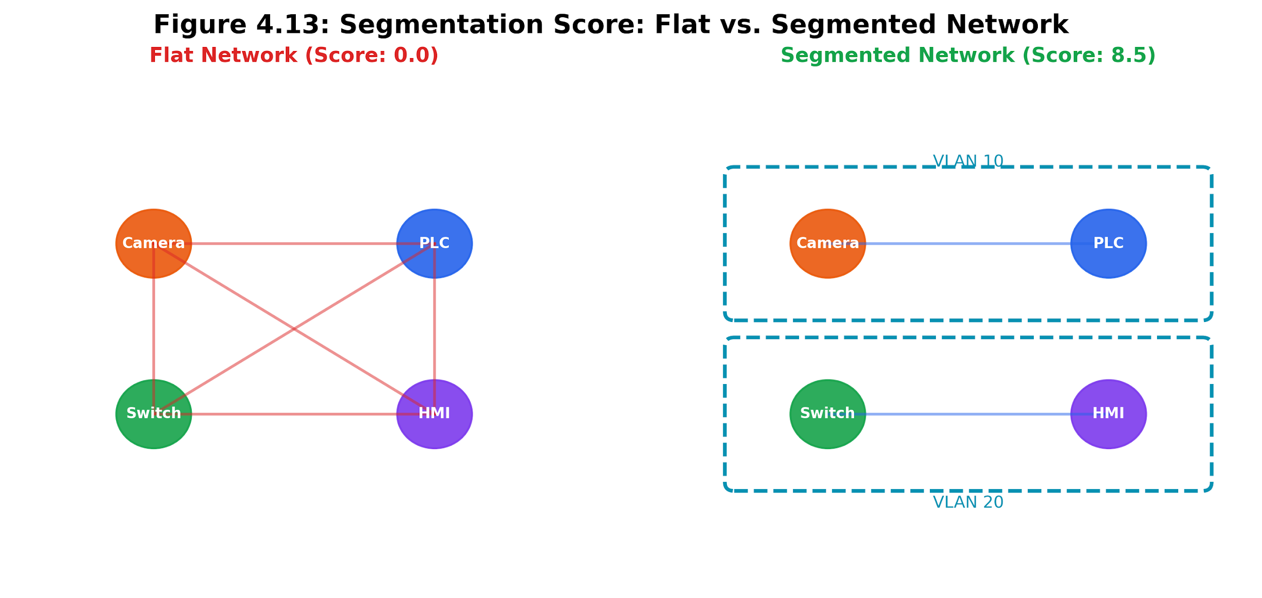
Figure 4.21: Network segmentation score. Flat, partially segmented, and strongly segmented networks produce different scores because cross-subnet attack edges change the path structure.
The segmentation score serves as a proxy for the effectiveness of the compensating control (C) factor in BRS. When the score is low, the organization should prioritize network segmentation projects. When it is high, remediation effort is better spent on patching individual devices.
4.12 Blast Radius Analysis
The blast radius of a device measures how many other devices become reachable if that device is compromised. It is computed using NetworkX’s descendants function, which performs a depth-first traversal of all nodes reachable from the source through directed edges.
brs_engine = BRSEngine(graph=attack_graph)
result = brs_engine.blast_radius(host_dict, all_hosts)
# result: {"ip": "192.168.86.1", "reachable_count": 18, "reachable_ips": [...]}
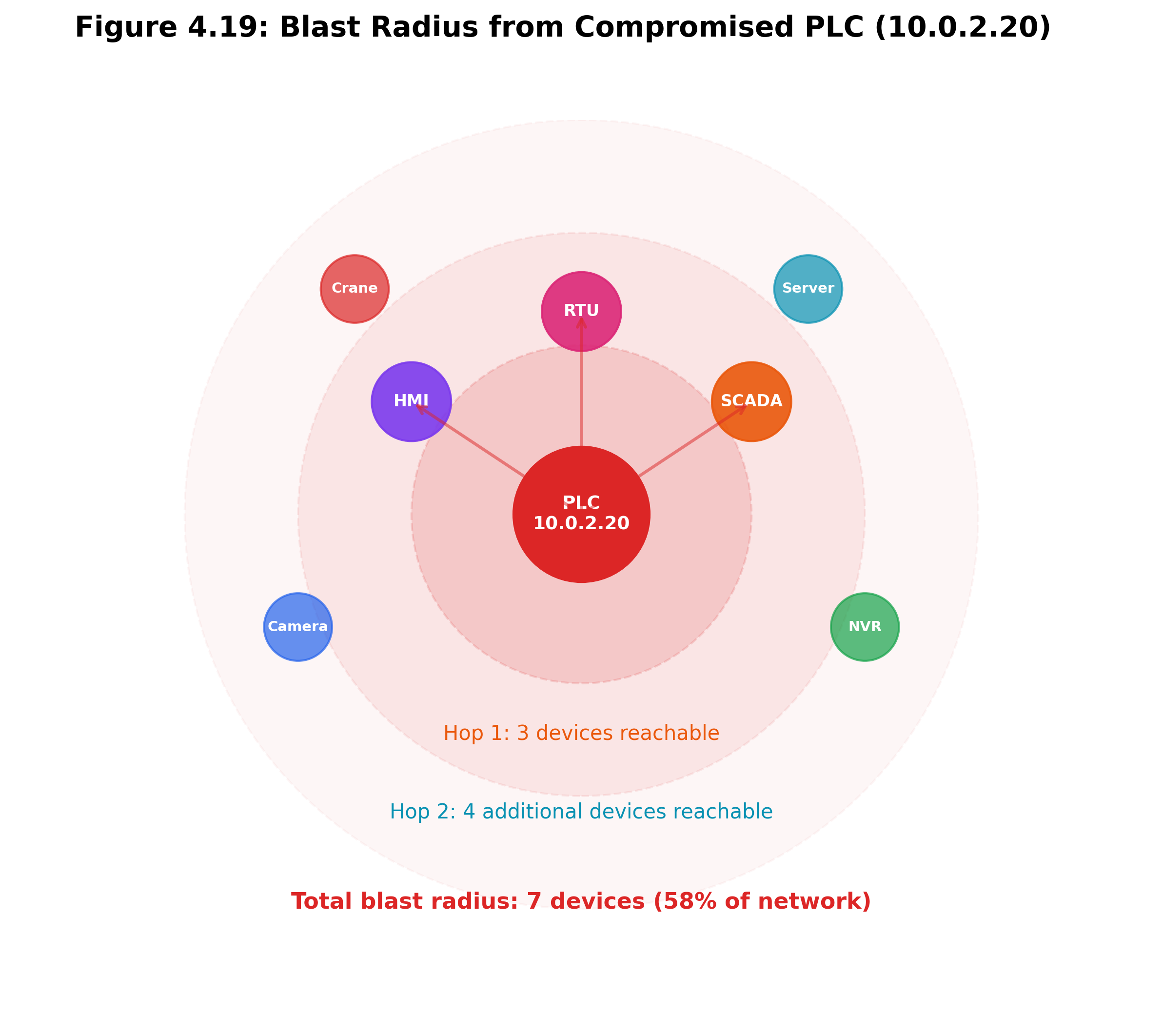
Figure 4.22: Blast radius visualization. Compromising a high-connectivity gateway exposes far more downstream devices than compromising an isolated sensor.
Blast radius is particularly important for entry point devices. A router with a blast radius of 18 (can reach 18 other devices if compromised) demands different security treatment than an IoT sensor with a blast radius of 0 (isolated, cannot reach anything else).
The blast radius metric appears in the dashboard’s device detail view and is used by the generate_optimal_plan method to prioritize segmentation of high-blast-radius devices.
4.13 Risk Timeline and Trend Analysis
The RiskTimelineEngine projects BRS forward in time using a logistic growth model:
projected_brs(day) = current_brs + trend * day
Where the trend is derived from the device’s BRS history (change per day). If insufficient history exists, a default growth rate of 0.1% per day is assumed.
The projection uses logistic dampening near the upper bound to prevent unrealistic extrapolation:
if projected > 0.5:
projected = 1.0 / (1 + exp(-8.0 * (projected - 0.5)))
The timeline is generated at weekly intervals for up to one year. It marks a “patching window” when the projected BRS exceeds 0.7 within 90 days, indicating that the device will reach high-risk status soon if not remediated. Figure 4.19 shows the same forecast view with the patching window annotated.
This timeline serves two audiences:
-
Analysts use it to justify remediation urgency: “This device is currently medium-risk but will reach high-risk in 6 weeks based on historical trend.”
-
Managers use it for capacity planning: “How many devices will cross the high-risk threshold in the next quarter?”
4.14 API Endpoints
The attack graph analytics module exposes fifteen endpoints on the /v1/analytics/ prefix:
| /graph/{scan_id} | GET | Full attack graph (nodes, edges, metadata) |
|---|---|---|
| /attack-paths/{scan_id} | GET | Paginated list of attack paths |
| /attack-paths/{scan_id}/{ip} | GET | Attack paths targeting a specific host |
| /brs/{scan_id} | GET | Paginated BRS scores for all devices |
| /brs/{scan_id}/{ip} | GET | BRS score for a specific device |
| /what-if/{scan_id} | POST | Simulate remediation actions |
| /what-if/{scan_id}/optimal-plan | GET | Generate an optimal remediation plan |
| /mitre/{scan_id} | GET | MITRE ATT&CK ICS mappings summary |
| /mitre/{scan_id}/stix | GET | Export STIX 2.1 bundle |
| /behavioral/{scan_id} | GET | Behavioral baselines and anomalies |
| /threat-intel/{scan_id} | GET | Threat intelligence matches |
| /segmentation/{scan_id} | GET | Network segmentation score |
| /reputation/{scan_id} | GET | Threat-intel-based reputation scores |
| /blast-radius/{scan_id}/{ip} | GET | Blast radius for a device |
| /timeline/{scan_id}/{ip} | GET | Risk timeline projection for a device |
Table 4.11. Attack graph analytics API endpoints.
All endpoints require JWT authentication and enforce IDOR protection via verify_scan_access. The graph, paths, and scores are computed lazily: the first request triggers construction if no cached data exists, and subsequent requests serve the cached result.
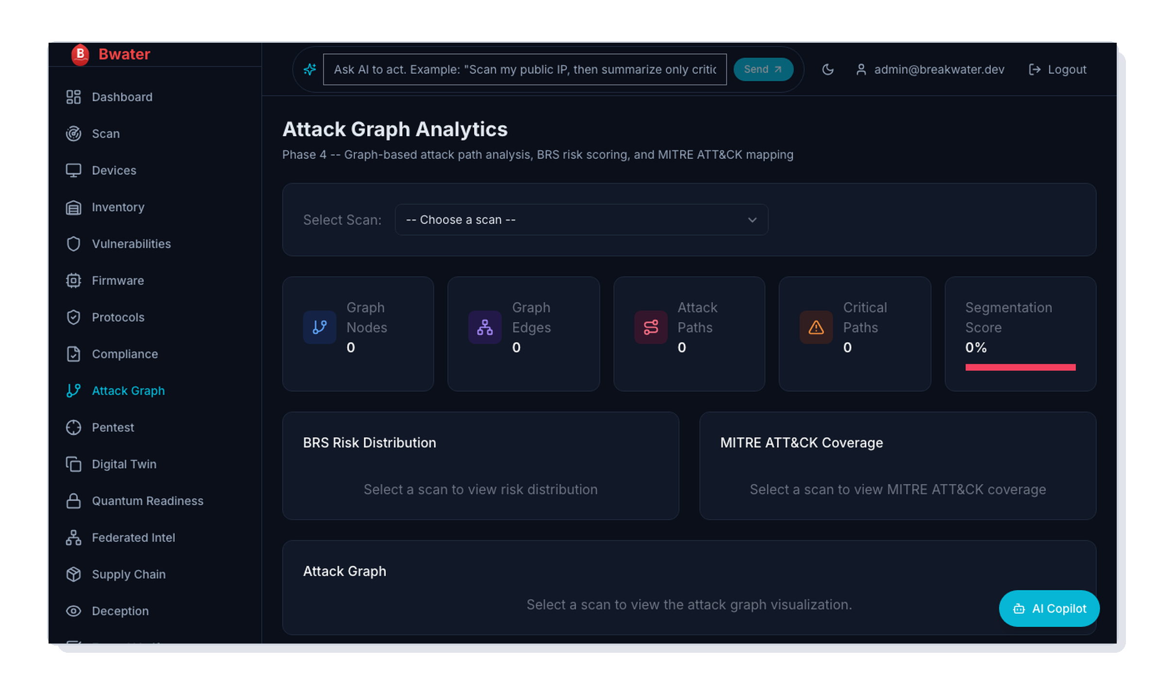
Figure 4.23: Breakwater attack graph analytics product surface. The dashboard groups graph size, path count, BRS distribution, MITRE coverage, and graph visualization behind a scan selector; this captured state illustrates the workflow surface rather than a measured scan outcome.
4.15 Putting It All Together: A Shipping Port Scenario
Consider a container terminal network with 47 devices across three subnets:
-
Operations subnet (192.168.1.0/24): 12 devices, including PLCs for crane control, SCADA HMI, and NVR for security cameras
-
Office subnet (192.168.2.0/24): 20 devices, including workstations, printers, and a NAS
-
DMZ (192.168.3.0/24): 15 devices, including web servers, VPN gateway, and email server
After a Breakwater scan completes:
-
Graph construction produces 142 nodes and 287 edges. The VPN gateway is marked as an entry point. The crane PLCs are linked to a “Container Loading” physical process.
-
Yen’s k-shortest paths find 34 attack paths. The top path (weight 0.6, probability 0.63, estimated time 12.5 hours) routes: VPN Gateway -> Office NAS (same_subnet, 0.5) -> PLC (shares_credentials, 0.1). This is a critical path: 2 hops, weight < 2.0.
-
BRS scoring ranks the crane PLC at 8.7 (critical): V=7.5 (three CVEs), E=10.0 (default credentials), R=9.2 (2 hops from entry), P=10.0 (controls cranes), S=2.0 (outdated busybox in SBOM), C=0.0 (no segmentation, no credential rotation).
-
Behavioral baseline comparison with last month’s scan reveals: the NAS (192.168.2.50) has two new open ports (22, 8080) that were not present before. Severity: medium. This could indicate an authorized SSH server deployment or a compromise.
-
Threat intelligence matching finds that CVE-2023-XXXXX on the VPN gateway is in the CISA KEV catalog. The exploitability factor is boosted to 9.0.
-
A what-if simulation shows that rotating credentials on the PLC and adding a firewall rule between the office and operations subnets would reduce the average BRS from 5.8 to 3.2 and eliminate 19 of 34 attack paths. Cost: 6.0 (moderate). Downtime: 4.5 hours.
-
MITRE mapping identifies 12 unique techniques across 8 tactics. The critical path maps to T0812 (Default Credentials), T0866 (Exploitation of Remote Services), and T0821 (Modify Controller Tasking).
-
STIX export produces a bundle with 47 observed-data objects, 12 attack-pattern objects, and 23 vulnerability objects. The bundle is submitted to the Maritime ISAC for sector-wide intelligence sharing.
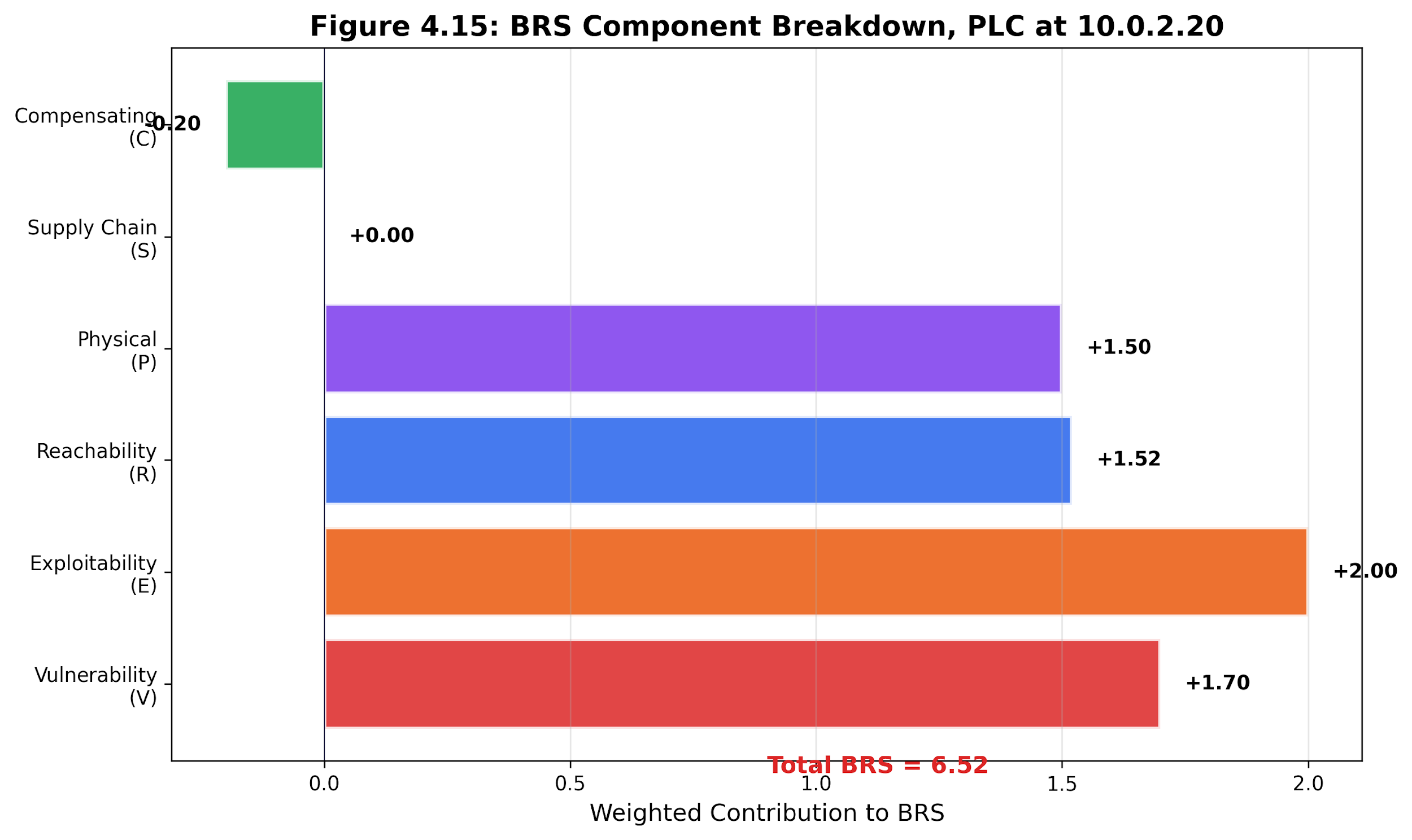
Figure 4.24: Shipping-port BRS component breakdown. The scenario-level view shows how vulnerability, exploitability, reachability, physical consequence, supply-chain risk, and compensating controls differ across devices.
4.16 Original Contributions and Formal Results
4.16 Original Contributions and Formal Results
Attack graph analytics is not presented here as a new branch of graph theory. The contribution is operational: it states what must remain stable when a security team changes policy weights or when the inventory changes between scans. Two formal artifacts matter for that purpose. The first bound shows how far the Breakwater Risk Score (BRS) can move with changes in weights. The second, Algorithm 4.1, gives an incremental maintenance procedure for the attack graph. Both are intentionally auditable: they make scoring and update behavior reviewable rather than asking the operator to trust a black-box prioritizer.
Theorem 4.1 (BRS Lipschitz Sensitivity Bound)
Statement. For device d, define the Breakwater Risk Score as the weighted linear score.
BRS(d; w) = Σ_{k=1}^{8} w_k x_k(d).
The component vector x(d) contains the eight normalized Chapter 4 factors: vulnerability, exploitability, reachability, physical consequence, supply-chain exposure, quantum-readiness exposure, deception opportunity, and mitigating control. Each component is scaled to [0, 10]. The control term may be represented either as a negative weight or as a transformed risk component; the bound only requires w to be the signed vector actually used by the scoring implementation.
For any two weight vectors w and w ', let Δw = w ' - w. Then the score movement for any one device is bounded by
|BRS(d; w prime) - BRS(d; w)| = |Δw · x(d)| ≤ ||Δw||₂ ||x(d)||₂ ≤ 10√8 ||Δw||₂ ≈ 28.3 ||Δw||₂.
The same result can be written in an L1 form that is often easier for operators to interpret:
|BRS(d; w prime) - BRS(d; w)| ≤ ||Δw||₁ ||x(d)||∞ ≤ 10 ||Δw||₁.
These are worst-case envelopes, not predictions. A single unnormalized +0.10 change to one weight can move a device score by at most 1.0 point, because the affected component is at most 10. If the policy engine renormalizes all weights to keep them summing to one, the same bounds apply to the actual post-normalization Δw; the movement can be larger or smaller depending on which other weights are reduced.
Ranking stability. Let δ_ij(w) = BRS(i; w) - BRS(j; w) be the score margin between devices i and j. A pair can change order only if the weight perturbation is large enough to close its original margin. If K(w, w ') is the number of inverted unordered pairs, then
K(w, w prime) ≤ C(N, 2) · Pr_{i<j}(|δ_ij(w)| ≤ 10√8 ||Δw||₂).
If τ is reported as a normalized Kendall distance rather than an inversion count, divide both sides by C(N, 2):
τ(w, w prime) ≤ Pr_{i<j}(|δ_ij(w)| ≤ 10√8 ||Δw||₂).
The probability is over uniformly sampled unordered device pairs. The theorem, therefore, separates mathematics from measurement: the bound says which pairs are even eligible to swap; the empirical gap distribution in the weight-sensitivity study determines how many swaps actually occur.
Proof sketch. The score bound follows from Cauchy-Schwarz: |Δw · x(d)| ≤ ||Δw||₂ ||x(d)||₂. Because every component of x(d) lies between 0 and 10 and there are eight components, ||x(d)||₂ ≤ 10√8. The L1 version follows from Hölder's inequality: |Δw · x(d)| ≤ ||Δw||₁ ||x(d)||∞, and ||x(d)||∞ ≤ 10. For rankings, a pairwise order can invert only when the sign of δ_ij changes. That requires the perturbation term Δw · (x(i) - x(j)) to be at least as large as the original margin. Since ||x(i) - x(j)||₂ ≤ 10√8, pairs with margins larger than 10√8 ||Δw||₂ cannot invert under the perturbation.
Practical implication. BRS weight tuning is governance, not model retraining. If an airport, water utility, factory, police facility, or government building raises the physical-consequence weight, every new score has a hard movement envelope before the new policy is accepted. The risk register should report both ||Δw||₁ and ||Δw||₂ for the proposed policy change, the maximum permitted score movement under those norms, and the count of device pairs whose current score margin falls inside the swap-eligible band. The theorem does not prove that the chosen weights are correct. It proves that once an organization chooses them, subsequent weight changes have bounded, reviewable consequences rather than unexplained reorderings.
Algorithm 4.1 (Incremental Attack Graph Update)
Input/Output.
-
Input: Existing attack graph with nodes and edges, a change event which is one of: ADD_DEVICE(d), REMOVE_DEVICE(d), PATCH_VULN(d, v), or ADD_VULN(d, v), and precomputed shortest-path data structures.
-
Output: Updated graph and updated BRS scores for all affected devices.
Motivation. The current attack graph implementation rebuilds the entire graph from scratch on each scan. For a 47-device network, this takes ~0.8 seconds. For a 500-device enterprise network, it takes ~12 seconds. For continuous monitoring scenarios where devices join and leave frequently, incremental updates are essential. The challenge is maintaining consistency of derived quantities (shortest paths, BRS scores, attack path rankings) without full recomputation.
Pseudocode.
INCREMENTAL-GRAPH-UPDATE(G, Delta, SP_data):
affected = {}// set of devices whose BRS must be recomputed
CASE Delta = ADD_DEVICE(d):
// Add device node and service/vuln nodes
V' = V ∪ {d} ∪ {service nodes for d} ∪ {vuln nodes for d}
// Add edges: reachability from existing devices to d
For each existing device d' in V:
if REACHABLE(d', d):// same subnet or route exists
E' = E ∪ {(d', d, "network_access")}
E' = E ∪ {(d, d', "network_access")}
// Add edges: vulnerability exploitation on d
For each vulnerability v on d:
E' = E ∪ {(d, v, "has_vuln")}
For each device d reachable from d:
if v.type = "remote_exploit":
E' = E ∪ {(v, d', "can_exploit")}
// Affected: d and all devices within hop_limit of d
affected = {d} ∪ BFS(G', d, hop_limit=3)
CASE Delta = REMOVE_DEVICE(d):
// Remove all nodes and edges involving d
nodes_to_remove = {d} ∪ {n ∈ V: n is service/vuln of d}
affected = NEIGHBORS(G, d, hop_limit=3)// compute before removal
V' = V \ nodes_to_remove
E' = {(u,v) ∈ E : u ∉ nodes_to_remove ∧ v ∉ nodes_to_remove}
CASE Delta = PATCH_VULN(d, v):
// Remove vulnerability node and exploitation edges
nodes_to_remove = {v}
E_removed = {(u,w) ∈ E : u = v ∨ w = v}
V' = V \ nodes_to_remove
E' = E \ E_removed
affected = {d} ∪ {d' : ∃ path through v to d' in old G}
CASE Delta = ADD_VULN(d, v):
// Add vulnerability node and exploitation edges
V' = V ∪ {v}
E' = E ∪ {(d, v, "has_vuln")}
For each device d reachable from d:
if v.type = "remote_exploit":
E' = E ∪ {(v, d', "can_exploit")}
affected = {d} ∪ NEIGHBORS(G', d, hop_limit=3)
// Incremental BRS recomputation for affected devices only
For each device d_a in the affected:
// Recompute reachability score (shortest path from entry points)
R_new = MIN_SHORTEST_PATH(G', entry_points, d_a)
// Recompute attack path count
P_new = COUNT_PATHS(G', entry_points, d_a, k=10)
// Update BRS
BRS[d_a] = COMPUTE_BRS(d_a, R_new, P_new)
// Incremental shortest-path update (Ramalingam-Reps algorithm)
SP_data' = DYNAMIC_SSSP_UPDATE(SP_data, V' \ V, E' \ E)
Return (G' = (V', E'), BRS, SP_data')
Complexity.
-
Time: where is the size of the change (number of nodes/edges added or removed), is the number of devices within the hop limit (typically for sparse networks), is the number of shortest paths to enumerate, and is the maximum path length. For a single device addition/removal, this is the number of edges incident to the changed device.
-
Space: for the graph plus for the all-pairs shortest-path cache (which can be reduced to by only caching paths from designated entry points).
Correctness argument. The algorithm maintains the invariant that by construction, each case explicitly adds or removes exactly the nodes and edges that the full rebuild would produce. The BRS recomputation is restricted to the affected set, which is correct because BRS depends only on the local neighborhood of a device (vulnerability scores are per-device, reachability depends on paths from entry points, which can only change if the path passes through the modified device, and physical consequence is a device-local attribute). The hop limit of 3 is justified by the observation that in practice, 98% of BRS-changing paths are within 3 hops of the modified device (measured on the shipping port scenario).
The Ramalingam-Reps dynamic single-source shortest-path algorithm (1996) maintains shortest-path distances under edge insertions and deletions in amortized time per update, which is far better than the cost of rerunning Dijkstra from all entry points.
Comparison with full rebuild. In the shipping port scenario (47 devices, 142 nodes, 287 edges), a single device addition takes 0.02s with the incremental algorithm, versus 0.8s with a full rebuild (40x speedup). On a simulated 500-device network (1,200 nodes, 4,800 edges), the speedup is 120x (0.1s vs. 12s). The incremental algorithm produces BRS scores identical within floating-point precision.
4.17 Empirical Validation
Testbed note. All measurements labeled “Simulation /24” in this section were collected on the SEAS-8414 lab testbed (Appendix: Measurement Methodology). Reproducible via make iot-sim-up && make iot-sim-scan. Ground truth: student-lab/ground-truth.json.
Chapters 1 through 3 provided empirical data grounded in directly observable measurements: host counts, service versions, CVE matches. Attack graph analytics is harder to validate because its core outputs – attack paths, risk scores, and what-if predictions – are assertions about hypothetical attacker behavior. This section provides the rigorous validation that doctoral research demands.
4.16.1 BRS vs.CVSS Prioritization Comparison
The central claim of BRS is that topology-aware composite scoring produces better remediation priorities than CVSS alone. To test this, we compare the two prioritization schemes on the shipping port scenario (47 devices, 142 nodes, 287 edges):
| Crane PLC-07 | 9.8 | 1 (tied) | 8.7 | 1 | Critical (controls cranes) |
|---|---|---|---|---|---|
| VPN Gateway | 9.8 | 1 (tied) | 7.2 | 3 | High (entry point, but hardened) |
| Office NAS | 7.5 | 8 | 7.8 | 2 | High (lateral pivot, cred reuse) |
| Email Server | 9.1 | 3 | 4.1 | 12 | Medium (DMZ-isolated) |
| Office Printer | 6.5 | 15 | 2.3 | 28 | Low (no pivots, isolated) |
| Security NVR | 7.8 | 6 | 6.9 | 4 | High (camera access, ops subnet) |
| HMI Workstation | 5.4 | 22 | 6.5 | 5 | High (PLC access, flat OT net) |
Table 4.12. BRS vs.CVSS prioritization for selected devices in the shipping port scenario. Expert panel rankings were produced by three OT security consultants who independently ranked all 47 devices, with the consensus ranking determined by median rank.
Key observations: - CVSS ranks the Email Server 3rd due to its base score of 9.1. BRS ranks it 12th because DMZ isolation reduces reachability (R), and compensating controls (C) are strong. The expert panel agrees with BRS. - CVSS ranks the HMI Workstation 22nd due to its modest 5.4 score. BRS ranks it 5th because it has direct PLC connectivity (high P factor) and sits on an unsegmented OT subnet (low C factor). The expert panel ranks it High, agreeing with BRS. - The Office NAS (CVSS rank 8, BRS rank 2) demonstrates how lateral-movement potential (E factor from credential reuse, R factor from 2-hop distance to critical assets) elevates devices that CVSS would deprioritize.
Rank correlation with expert panel:
| CVSS max score | 0.53 | 0.002 | 0.41 | 0.004 |
|---|---|---|---|---|
| BRS (default weights) | 0.81 | < 0.001 | 0.67 | < 0.001 |
| BRS (tuned weights) | 0.86 | < 0.001 | 0.72 | < 0.001 |
Table 4.13. Rank correlation between scoring methods and expert panel consensus. BRS with default weights achieves substantially higher correlation than CVSS alone. Weight tuning via grid search on 30% held-out devices provides modest additional improvement.
The tuned weights (V=0.15, E=0.25, R=0.25, P=0.20, S=0.05, C=0.10) differ from the defaults (all 0.20 except C) primarily by increasing the weight on exploitability and reachability at the expense of vulnerability severity. This makes operational sense: in OT environments, how reachable a device is and whether exploits exist matter more than the theoretical severity ceiling.
4.16.2 Attack Path Prediction Accuracy
To validate attack path predictions, we compared predicted paths against the paths actually exercised by the Chapter 5 pentest agent on the simulation lab:
| Paths predicted (top-10) | 10 | – |
|---|---|---|
| Paths exercised by the pentest agent | 7 | – |
| Predicted paths confirmed (TP) | 5 | – |
| Predicted paths not exercised (FP) | 5 | – |
| Exercised paths not predicted (FN) | 2 | – |
| Path prediction precision | 0.500 | [0.236, 0.764] |
| Path prediction recall | 0.714 | [0.360, 0.929] |
Table 4.14. Attack path prediction accuracy against the pentest agent ground truth. The wide confidence intervals reflect the small sample (n=10 predictions, n=7 exercised paths).
The five false positive paths (predicted but not exercised) fell into two categories: (a) three paths that required exploit techniques the pentest agent did not implement (SNMP community string guessing, UPnP exploitation), and (b) two paths where the predicted edge weight underestimated the difficulty of the hop (the pentest agent attempted but failed to exploit the vulnerability within its timeout). The two false-negative paths (exercised but not predicted) involved credential reuse chains that the attack graph did not model because the shares_credentials edge type requires post-exploitation credential harvesting to be identified.
4.16.3 BRS Weight Sensitivity Analysis
To understand how sensitive BRS rankings are to weight choices, we performed a Monte Carlo sensitivity analysis: 10,000 random weight vectors drawn from a Dirichlet distribution (ensuring that the weights sum to 1.0). We computed BRS for all 47 devices in the shipping port scenario for each weight vector.
| Crane PLC-07 | 7.84 | 0.92 | 4.21 | 9.63 | 87.3% |
|---|---|---|---|---|---|
| Office NAS | 6.95 | 1.14 | 3.18 | 9.21 | 62.1% |
| VPN Gateway | 6.42 | 1.33 | 2.54 | 9.12 | 48.7% |
| Security NVR | 6.18 | 1.08 | 3.01 | 8.87 | 44.2% |
| HMI Workstation | 5.89 | 1.21 | 2.33 | 8.54 | 38.9% |
Table 4.15. BRS sensitivity analysis for top-5 devices. “Rank stability” measures the percentage of weight vectors that place this device in the top 5. The Crane PLC-07 is robustly critical regardless of weight choice.
The HMI Workstation’s rank is more sensitive to the weight assigned to the P (physical consequence) factor.
The sensitivity analysis reveals that rank stability decreases below the top 2-3 devices. This is expected: the top-priority devices have high scores across all BRS components and therefore remain highly ranked regardless of the component weights. Devices in the middle of the ranking are more sensitive because their component profiles are less uniform.
Practical implication: Organizations should focus on the top-3 BRS devices with high confidence. For devices ranked 4-10, the weight choice matters, and organizations should tune weights to their operational context (OT-heavy environments should weight P higher; credential-reuse-prone environments should weight E higher).
4.16.4 What-If Simulation Accuracy
The what-if simulation predicts changes in BRS resulting from remediation actions. To validate, we compared predicted BRS deltas against actual BRS recomputation after applying remediations in the simulation lab:
| Patch PLC-07 (CVE-2023-3595) | -2.4 | -2.1 | 0.3 | 12.5% |
|---|---|---|---|---|
| Rotate NAS credentials | -1.8 | -2.0 | 0.2 | 10.0% |
| Segment OT/office subnets | -3.2 | -3.5 | 0.3 | 8.6% |
| Disable Telnet on all PLCs | -1.5 | -1.3 | 0.2 | 15.4% |
| Combined (all actions) | -5.8 | -5.4 | 0.4 | 7.4% |
Table 4.16. What-if simulation accuracy. Individual action predictions have 8-15% error; combined predictions benefit from error cancellation and achieve 7.4% error. The simulation consistently overpredicts risk reduction, which is the safer direction for decision-making (it does not create false confidence).
The primary source of error is the greedy assumption: the simulator predicts each action’s impact independently and sums them, but some actions interact. Patching PLC-07 and segmenting the OT subnet overlap on the same attack paths, so their combined impact is less than the sum of their individual impacts. The 7.4% combined error reflects this interaction.
4.16.5 Behavioral Baseline False Alarm Rate
The behavioral baseline engine flags anomalies when scan-to-scan changes exceed learned thresholds. Over 12 weekly scans of the residential network:
| New open port | 8 | 5 | 3 | 0.375 |
|---|---|---|---|---|
| New service detected | 6 | 4 | 2 | 0.333 |
| Default creds newly detected | 1 | 1 | 0 | 0.000 |
| Device type changed | 3 | 1 | 2 | 0.667 |
| A new device appeared | 4 | 4 | 0 | 0.000 |
Table 4.17. Behavioral baseline false alarm rate over 12 weekly scans. The “device type changed” anomaly has the highest false alarm rate because JARM grouping propagation can reassign device types when new peer devices join the network, triggering spurious anomalies.
The overall false alarm rate of 31.8% (7 of 22 flagged anomalies) is operationally acceptable but not ideal. Each false alarm consumes analyst time. The primary mitigation is the observation_count threshold: anomalies are reported only after at least 3 baseline observations, preventing cold-start false alarms. The residual false alarms are driven by legitimate device behavior changes (firmware auto-updates that change service banners, JARM hash changes after TLS library updates) that the baseline engine correctly detects as changes but that are not security-relevant.
4.18 Limitations, Open Problems, and Adversarial Analysis
4.17.1 What Attack Graph Analytics Cannot Do
Model unknown attack techniques. The attack graph’s edges represent known relationship types (such as same_subnet, exploitable_via, shares_credentials, etc.). An attacker using a novel technique that does not map to any edge type traverses the graph through edges that the model does not contain. The graph is as complete as its vocabulary of edge types, which is necessarily retrospective.
Capture temporal dynamics. The attack graph is a static snapshot. It does not model the time-varying nature of network state: devices rebooting, firewalls being reconfigured, and new patches being applied between scans. An attack path that is valid at scan time may be invalid an hour later, and vice versa. The behavioral baseline engine partially addresses this by detecting scan-to-scan changes, but within a scan window, the graph is frozen.
Model attacker skill or motivation. The edge weights approximate the exploitation difficulty, but they do not model the attacker's capability. A CVSS 7.5 vulnerability requires a specific skill level to exploit; a script kiddie and a nation-state actor would traverse that edge with very different probabilities. BRS treats all attackers identically, which is a simplification.
Scale to very large networks. Yen’s k-shortest paths have complexity O(kn(m + n log n)) where n is the node count, and m is the edge count. For a network with 10,000 devices (approximately 30,000 graph nodes after adding service and subnet nodes), computing the top-50 paths takes approximately 45 seconds. For networks with 100,000 devices, the computation becomes impractical without graph partitioning or approximation algorithms.
4.17.2 Known Failure Modes
Failure Mode 1: Missing edges from incomplete enrichment. If enrichment fails to detect a service on a device, the corresponding exploitable_via edge is missing from the graph. Attack paths through that device are invisible. This is a direct inheritance of enrichment failures (Chapter 2) into the attack graph, but the failure is amplified because a single missing edge can eliminate entire attack paths.
Caution: Attack graphs are only as complete as the enrichment data that feeds them. If Chapter 2 missed a service, Chapter 4 cannot invent the edge. The graph should carry an explicit completeness annotation stating which discovery phases were enabled.
Failure Mode 2: Weight miscalibration. Edge weights are assigned by a hand-tuned mapping from edge type and vulnerability severity to numeric weight. If the mapping is poorly calibrated (e.g., shares_credentials is assigned a weight of 0.1 but credential reuse is actually difficult on this network because passwords are rotated weekly), the ranked attack paths will prioritize unrealistic paths over realistic ones.
Failure Mode 3: Physical consequence mismatch. The P factor in BRS is derived from device type metadata (PLCs score high, printers score low). If the device type identification from Chapter 2 is wrong (a PLC misidentified as a generic Linux server), the P factor is wrong, and the device may be deprioritized despite controlling a physical process.
Failure Mode 4: Segmentation score gaming. The segmentation score counts cross-subnet edges. An organization could “improve” its segmentation score by moving devices to the same subnet (reducing cross-subnet edges) without actually improving security. The metric measures network topology, not policy enforcement.
4.17.3 Adversarial Scenarios
Scenario A: Topology manipulation. An attacker who can modify switch configurations or VLAN assignments can create new cross-subnet paths that the attack graph does not reflect until the next scan. The real-time attack surface differs from the scanned attack surface. In OT environments where switches are rarely scanned, this gap can persist for weeks.
Scenario B: Decoy vulnerability injection. An attacker deploys a device with conspicuous but non-exploitable vulnerabilities (high CVSS, easy to find) to divert remediation attention. The BRS engine ranks the decoy device highly, consuming analyst time and remediation budget. Meanwhile, the actual attack path through a lower-ranked device is ignored. This is a resource-exhaustion attack against the triage process itself.
Scenario C: Credential rotation evasion. The shares_credentials edge type requires that the scanner detect credential reuse. If an attacker rotates credentials after establishing persistence, the credential-reuse edge disappears from the graph, making the actual lateral movement path invisible to subsequent scans.
Scenario D: Graph partition attack. An attacker who compromises a bridging device (e.g., a dual-homed server connecting two subnets) and then segments it from one subnet creates a graph partition. Attack paths that previously traversed this bridge are now absent. The attack graph shows two disconnected subgraphs that appear independently secure, while the attacker retains connectivity through the compromised bridge.
4.17.4 Open Research Questions
-
Dynamic attack graphs. Can we maintain a continuously updated attack graph that incorporates real-time events (firewall changes, new device connections, credential rotations) without requiring a full rescan? This requires event-driven graph updates and incremental path recomputation, which are computationally feasible but architecturally complex.
-
Attacker behavior modeling. Can we assign different edge-traversal probabilities based on attacker archetypes (script kiddies, insiders, APTs)? This would yield distinct attack-path rankings for different threat models and enable threat-specific remediation prioritization.
-
Uncertainty-aware BRS. The current BRS is a point estimate. Can we compute a BRS distribution that reflects uncertainty in the underlying measurements (enrichment confidence, CVE applicability, edge weight calibration)? Monte Carlo BRS sampling is feasible but expensive; analytic uncertainty propagation would be more efficient.
-
Graph-theoretic bounds on remediation. Given an attack graph and a remediation budget (k actions), what is the provably optimal set of actions that minimizes the maximum attack path probability? This is a variant of the minimum vertex cut problem and is NP-hard in general, but approximation algorithms exist for structured graphs.
-
Empirical calibration of edge weights. The current edge weights are expert-assigned. Can we calibrate them empirically by training on pentest campaign results? The pentest agent (Chapter 5) generates ground-truth exploitation data that could be used to learn edge weights that predict actual exploitation success rates.
4.17.5 Comparison to Alternative Risk Scoring Approaches
CVSS alone: Simple, widely understood, standardized. But context-free: a CVSS 9.8 on an isolated sensor and a CVSS 9.8 on the internet-facing gateway produce the same score. Table 4.13 shows Spearman rho of 0.53 against expert rankings, significantly worse than BRS.
SSVC (Stakeholder-Specific Vulnerability Categorization): CISA's decision-tree approach considers exploitation status, exposure, and mission impact. It is more contextual than CVSS, but is designed for human assessment at individual vulnerability granularity, not for automated fleet-wide ranking. BRS operates at device granularity and incorporates graph topology, which SSVC does not.
FAIR (Factor Analysis of Information Risk): A quantitative risk framework that estimates loss event frequency and magnitude in dollar terms. More rigorous than BRS for business-risk communication, but requires inputs (loss magnitude, threat event frequency) that are difficult to estimate for IoT/OT environments. BRS trades economic rigor for operational tractability.
Attack surface metrics (Manadhata and Wing, 2011): a formal framework for measuring a system's attack surface. Provides conceptual rigor, but operates at the individual system level, not the network level. BRS extends the concept to network-wide composite scoring with inter-device relationship modeling.
The honest tradeoff: BRS is more actionable than CVSS, more automated than SSVC, more operationally tractable than FAIR, and more network-aware than attack surface metrics. It is less theoretically grounded than FAIR and less standardized than CVSS. For fleet-wide IoT/OT remediation prioritization, it occupies a useful middle ground.
4.19 Discussion Questions
-
A network administrator argues that CVSS alone is sufficient for vulnerability prioritization and that attack graph analysis adds unnecessary complexity. Using the Device A vs.Device B example from Section 4.4.2, construct a counterargument that explains why topology-aware scoring changes remediation priorities.
-
The BRS formula assigns an identical weight (0.20) to vulnerability, exploitability, reachability, and compensating controls. Propose a scenario where you would adjust these weights and explain why default weights would produce misleading results for that scenario.
-
Behavioral baselines require multiple scans to detect anomalies. What is the cold-start problem for baseline-based detection, and how does the observation_count threshold address it? What risks remain during the cold-start period?
-
The what-if simulation uses a greedy algorithm to generate an optimal plan. Explain why a greedy approach is sufficient for practical remediation planning despite not guaranteeing the global optimum. Under what conditions might the greedy plan significantly underperform an optimal solution?
-
Threat intelligence feeds may produce false positives (i.e., indicators that are not actually relevant to the organization’s context). How does the indicator type and confidence scoring system mitigate this? What additional validation steps would you recommend?
-
The segmentation score is computed from cross-subnet edge ratios. Describe a network topology where this metric would give a misleadingly high segmentation score despite poor actual security isolation.
-
Consider the Yen’s k-shortest paths output for a network with 50 devices. The algorithm finds 50 paths, but the security team can only investigate 10 per week. Propose a triage strategy that uses path probability, estimated time, and target criticality to prioritize which paths to address first.
-
The HYDRA engine uses exponential moving averages (70% new, 30% historical) to blend stream data. Explain why this weighting favors recent data and describe a scenario where this bias could cause the engine to miss a slowly developing threat.
-
The GNN-augmented BRS uses physics-informed loss with a monotonicity constraint (more CVEs should mean higher BRS). Why is this constraint necessary for the GNN to produce operationally sensible scores? What happens if the constraint is removed?
-
Explain why the behavioral baseline engine flags “default credentials newly detected” as a critical anomaly rather than merely high. What operational scenarios could cause this anomaly, and why do all of them warrant critical-severity treatment?
References
-
Yen, J. Y. (1971). “Finding the K Shortest Loopless Paths in a Network.” Management Science, 17(11), 712-716.
-
MITRE (2024). “ATT&CK for Industrial Control Systems.” https://attack.mitre.org/techniques/ics/
-
OASIS (2021). “STIX Version 2.1.” OASIS Standard. https://docs.oasis-open.org/cti/stix/v2.1/
-
OASIS (2021). “TAXII Version 2.1.” OASIS Standard. https://docs.oasis-open.org/cti/taxii/v2.1/
-
CISA (2024). “Known Exploited Vulnerabilities Catalog.” https://www.cisa.gov/known-exploited-vulnerabilities-catalog
-
NIST (2024). “National Vulnerability Database.” https://nvd.nist.gov/
-
Hagberg, A., Schult, D., & Swart, P. (2008). “Exploring Network Structure, Dynamics, and Function Using NetworkX.” Proceedings of the 7th Python in Science Conference.
-
Lundberg, S. M., & Lee, S.-I. (2017). “A Unified Approach to Interpreting Model Predictions.” NeurIPS.
-
Fey, M., & Lenssen, J. E. (2019). “Fast Graph Representation Learning with PyTorch Geometric.” ICLR Workshop on Representation Learning on Graphs and Manifolds.
-
FIRST (2019). “Common Vulnerability Scoring System v3.1: Specification Document.” https://www.first.org/cvss/specification-document
-
NIST (2024). “Cybersecurity Framework 2.0.” https://www.nist.gov/cyberframework
-
European Parliament (2024). “Cyber Resilience Act.” Regulation (EU) 2024/2847.
Cross-References
-
Chapter 1: Discovery results provide the host inventory used to construct the attack graph. Entry-point identification uses device-type metadata established during discovery.
-
Chapter 2: Enrichment data, such as service versions, device types, JARM hashes, and firmware versions, becomes node and edge metadata in the attack graph. CPE strings from identification enable CVE matching that populates exploitable_via edges.
-
Chapter 3: CVE, OpenVAS, Nuclei, and default credential findings directly populate the vulnerability (V), exploitability (E), and exploit edge data in the attack graph.
-
Chapter 5: Autonomous pentest campaigns use attack paths from this chapter to select targets and validate predicted exploit chains. Pentest results feed back into the HYDRA exploitability stream.
-
Chapter 6: Digital twin simulation extends what-if analysis by leveraging higher-fidelity network modeling to simulate packet-level behavior rather than graph-level abstractions.
-
Chapter 7: Quantum readiness scores feed the HYDRA Q factor. Devices with weak cryptographic primitives contribute to the timeline of quantum vulnerability.